library(tidyverse)
library(vdemlite)
library(broom)
library(purrr)

# Load V-Dem data for 2019
model_data <- fetchdem(
  indicators = c("v2x_libdem","e_gdppc","v2cacamps"),
  start_year = 2019, end_year = 2019
) |>
  rename(
    country = country_name,
    lib_dem = v2x_libdem,
    wealth = e_gdppc,
    polarization = v2cacamps
  ) |>
filter(!is.na(lib_dem), !is.na(wealth))Least Squares Regression
November 6, 2025
Where is the prediction line? Example 1
[1] "r = 0.99"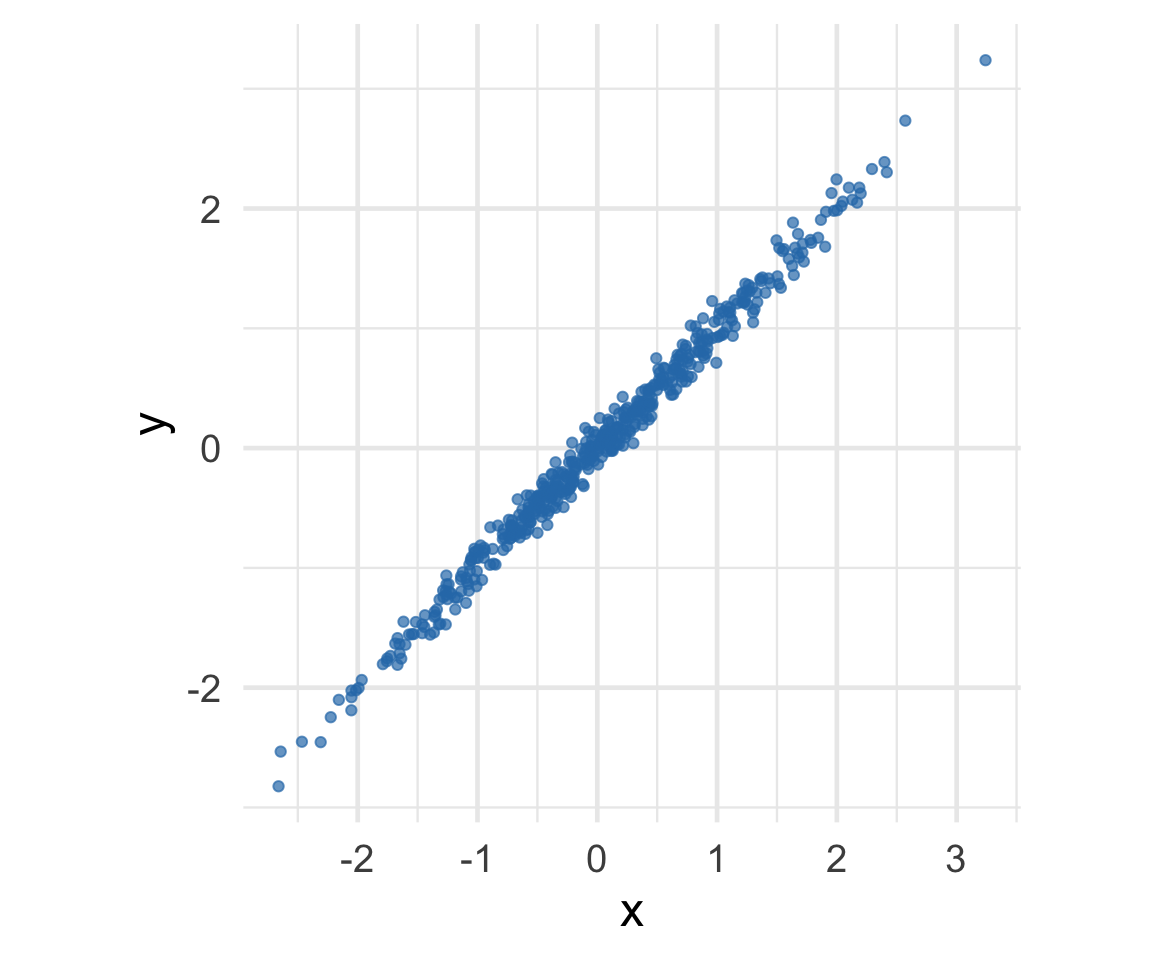
Where is the prediction line? Example 2
[1] "r = -0.06"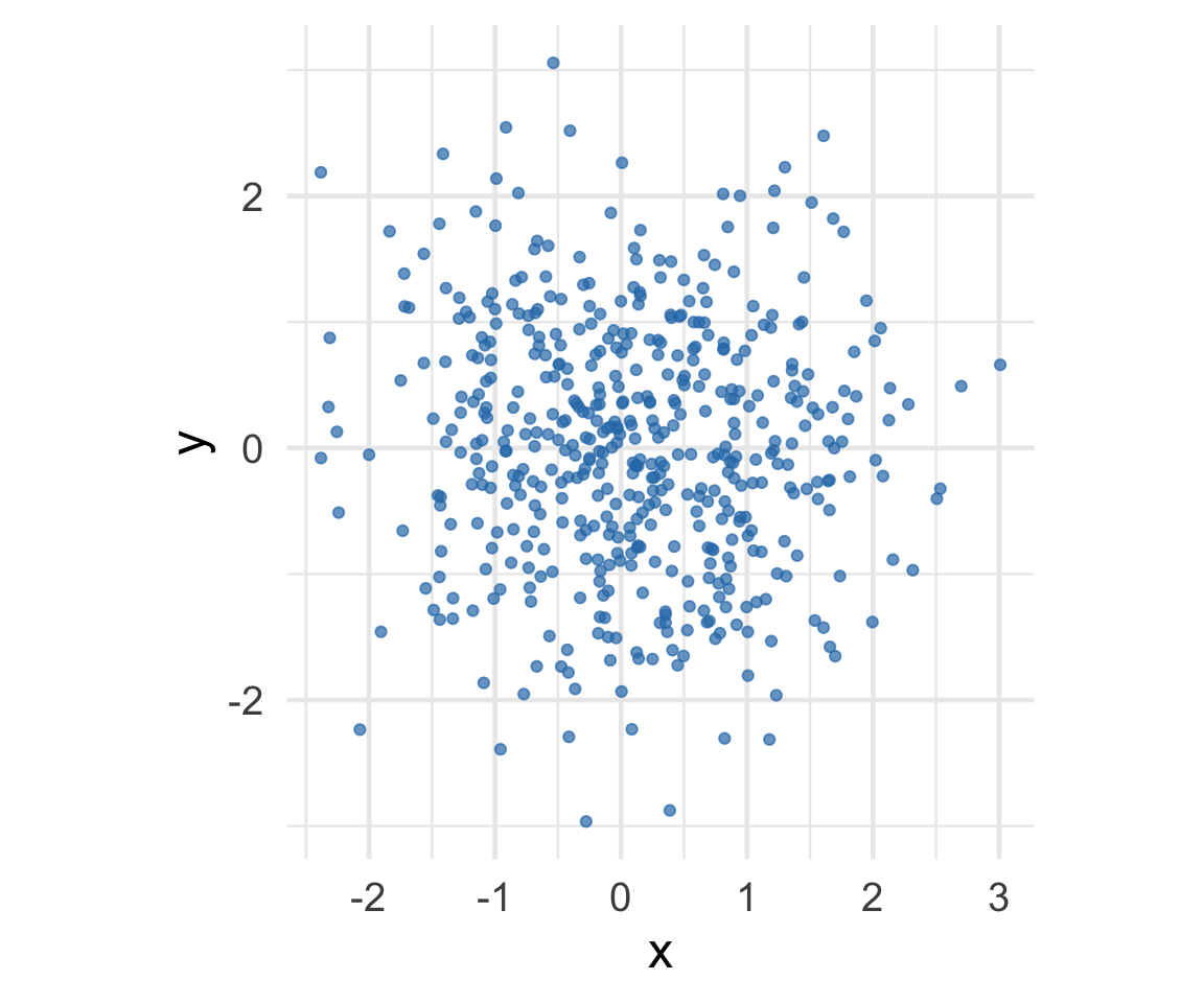
Where is the prediction line? Example 3
[1] "r = 0.66"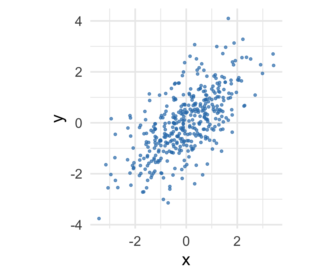
Which line is best?
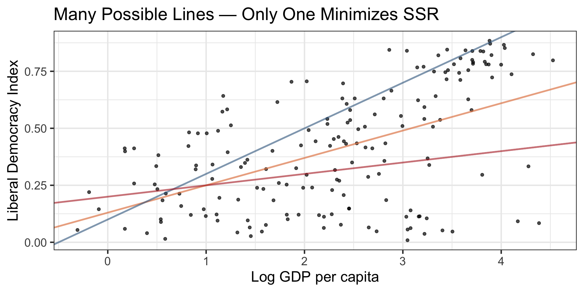
Worked Example: Democracy and GDP
Let’s compare several candidate lines on the V‑Dem data and compute their SSR.
Code
# Different lines parameters
test_lines <- tibble(
  intercept = c(0.13, 0.13, 0.13, 0.00),
  slope = c(0.12, 0.15, 0.08, 0.12),
  description = c("Least squares", "Steeper slope", "Gentler slope", "Different intercept")
)

# Visualize
ggplot(model_data, aes(x = log(wealth), y = lib_dem)) +
  geom_point(alpha = 0.6) +
  geom_abline(aes(intercept = intercept, slope = slope, color = description),
              data = test_lines, size = 1) +
  labs(x = "Log GDP per capita", y = "Liberal Democracy Index",
       title = "Comparing different possible regression lines",
       color = "Line type") +
  theme_bw(base_size = 18)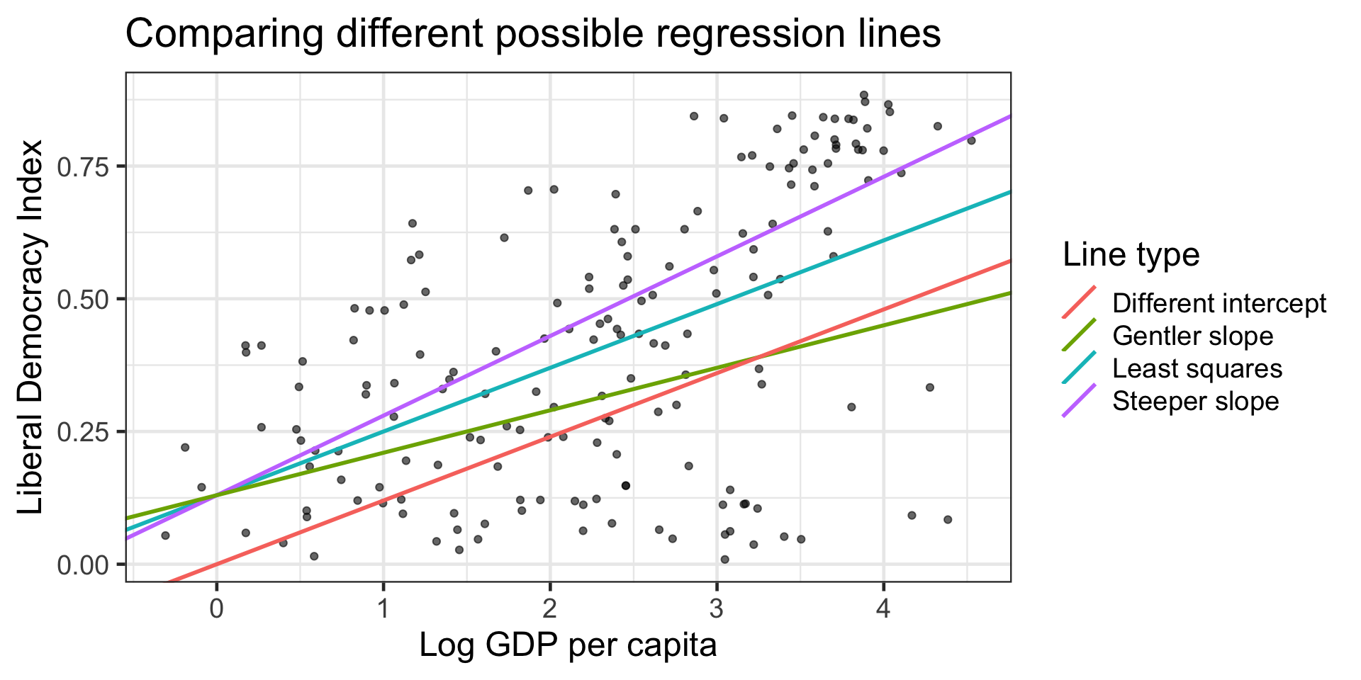
Least squares line (intercept = 0.13, slope = 0.12): SSR = 8.57
Steeper slope line (intercept = 0.13, slope = 0.15): SSR = 9.58
Gentler slope line (intercept = 0.13, slope = 0.08): SSR = 10.49
Different intercept line (intercept = 0.00, slope = 0.12): SSR = 11.58
Example: Shotput
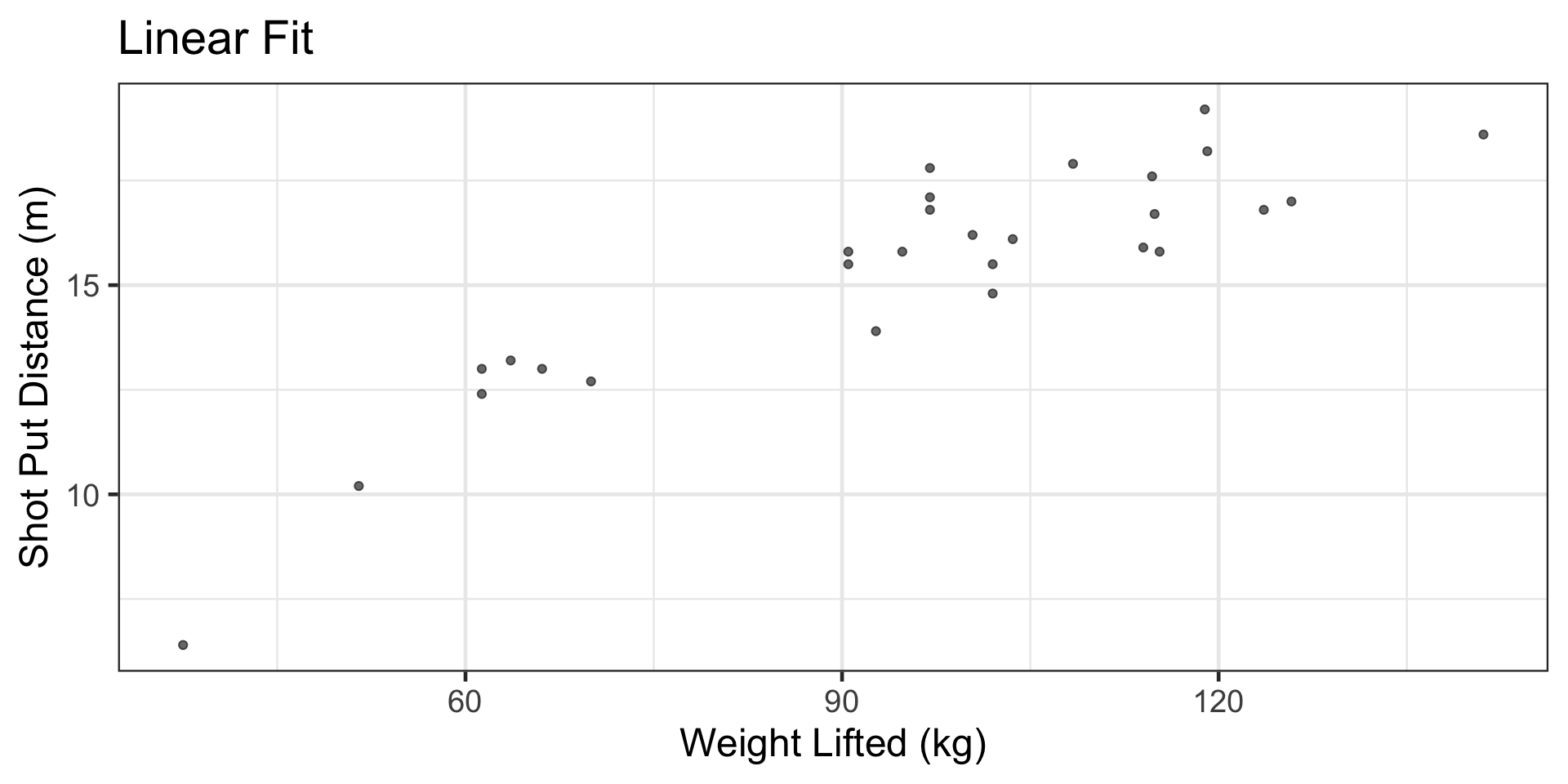
Example: Shotput
Compare linear vs. nonlinear fit visually
Code
p1 <- ggplot(shotput, aes(x = `Weight Lifted`, y = `Shot Put Distance`)) +
  geom_point(alpha = 0.6) +
  geom_line(data = aug_lin, aes(y = .fitted), color = "#8E2C90", linewidth = 1) +
  labs(
    title = "Linear Fit",
    x = "Weight Lifted (kg)",
    y = "Shot Put Distance (m)"
  ) +
  theme_bw(base_size = 18)

p2 <- ggplot(shotput, aes(x = `Weight Lifted`, y = `Shot Put Distance`)) +
  geom_point(alpha = 0.6) +
  geom_line(data = aug_quad, aes(y = .fitted), color = "steelblue4", linewidth = 1) +
  labs(
    title = "Quadratic Fit",
    x = "Weight Lifted (kg)",
    y = "Shot Put Distance (m)"
  ) +
  theme_bw(base_size = 18)

library(patchwork)
p1 + p2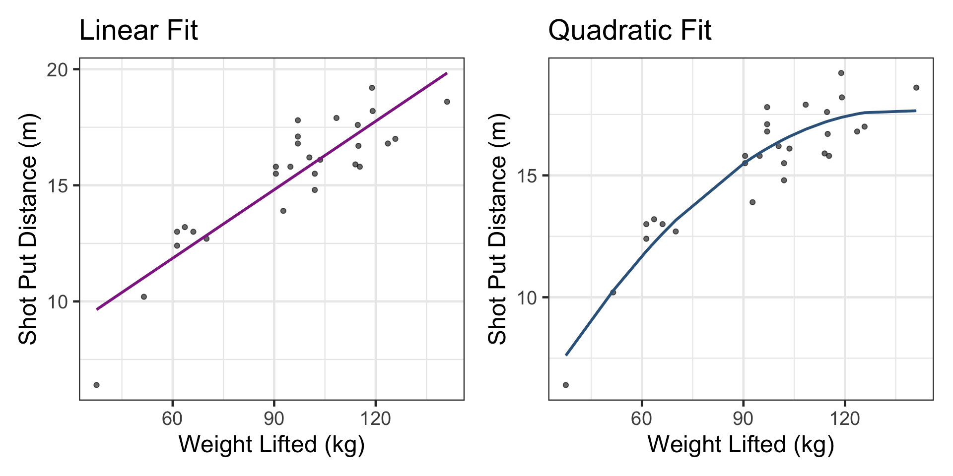
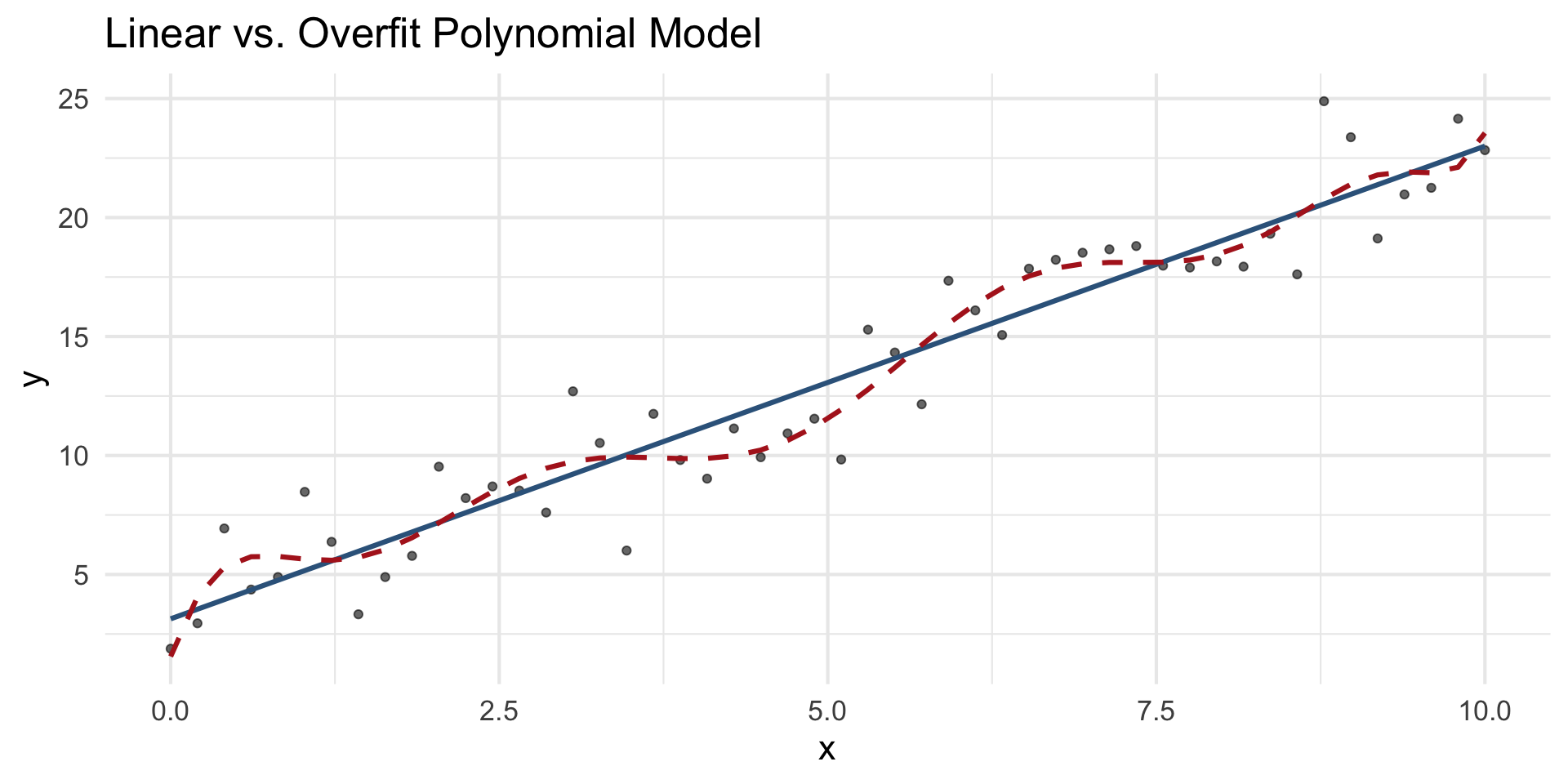
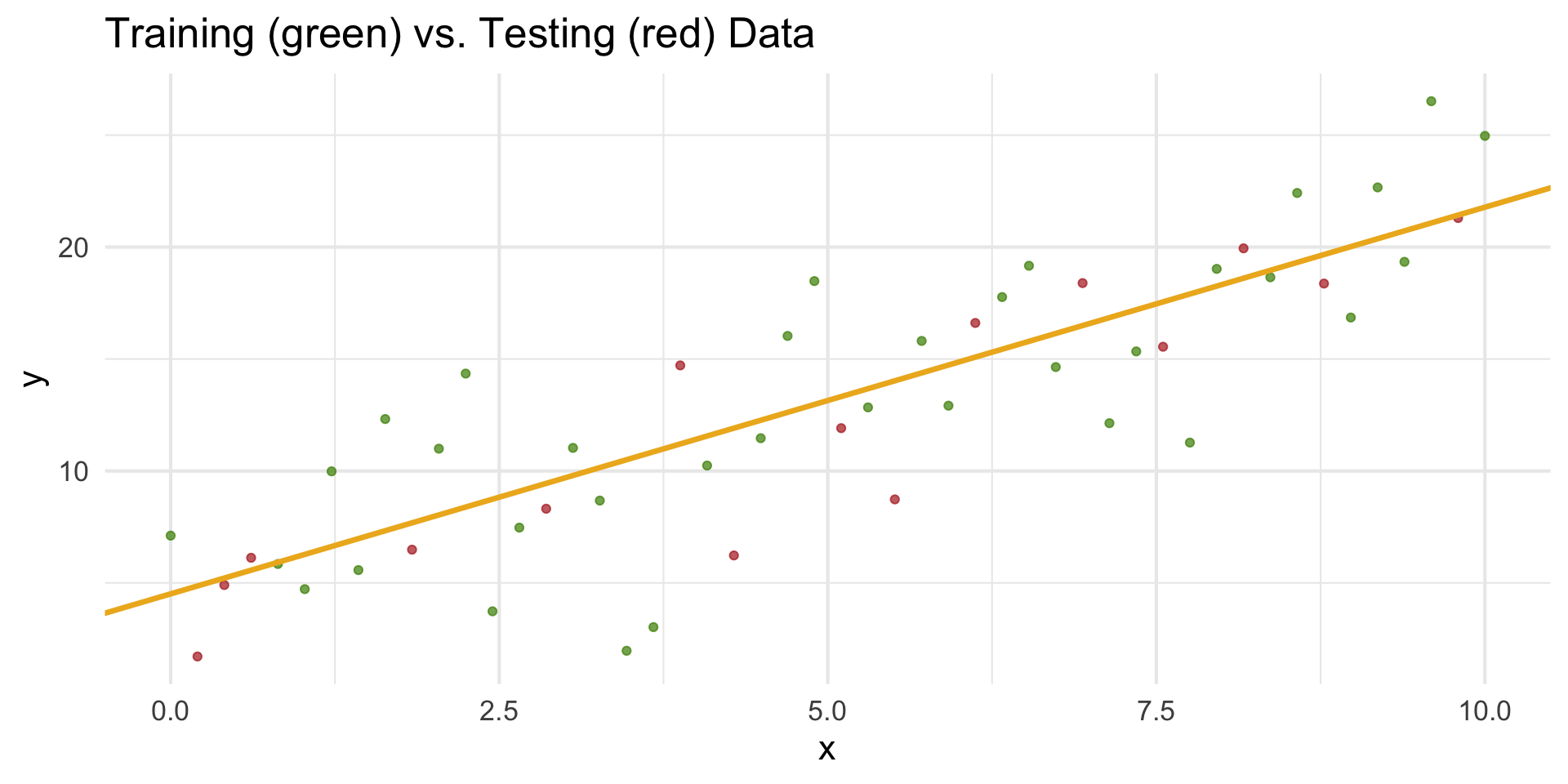
Beyond Fit: Training vs. Testing Data
- A model that fits the training data extremely well may not perform well on new data.
- Training data: used to estimate the model parameters (fit).
- Testing data: used to evaluate how well the model generalizes.
Overfitting vs. Underfitting