Machine Learning

November 20, 2025

Classifiers

The Google Science Fair

• Brittany Wenger, a 17-year-old high school student in 2012
• Won by building a breast cancer classifier with 99% accuracy

Breast Cancer Data

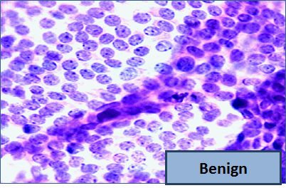
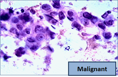
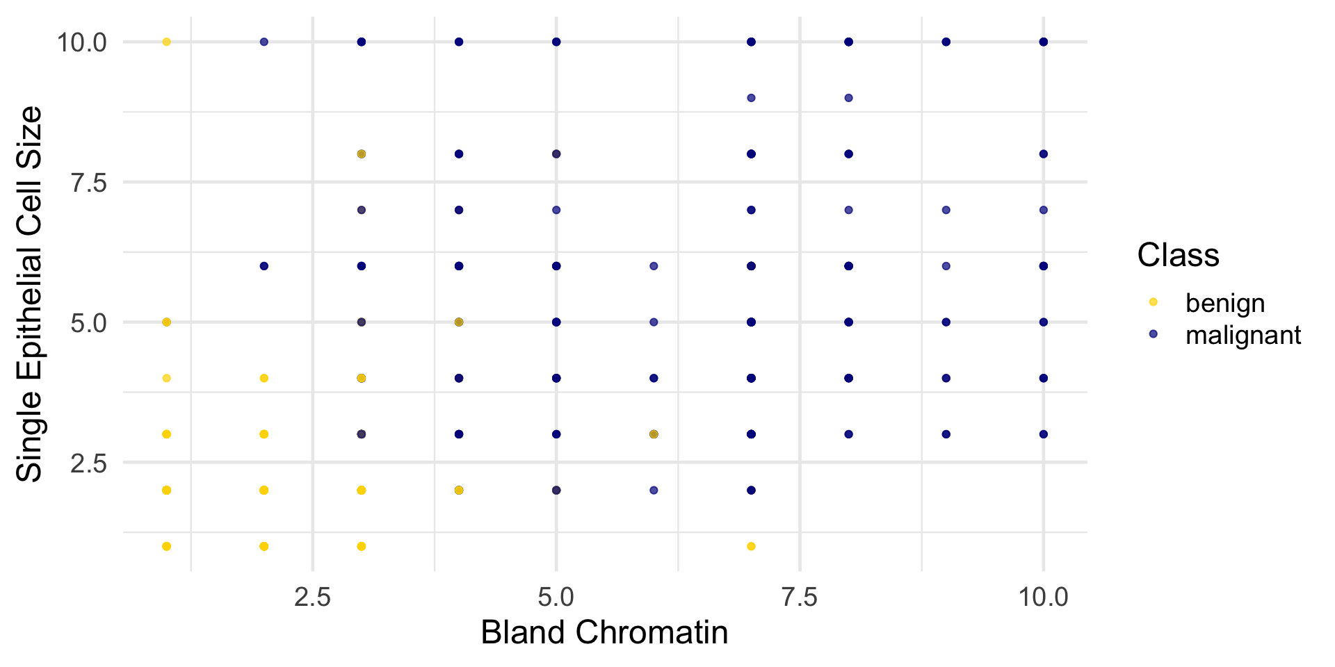
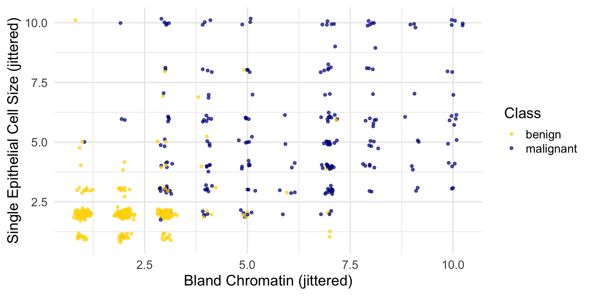
Our dataset contains attributes for cancer diagnosis: malignant (cancer) or benign (not cancer).

library(tidyverse)
library(tidymodels)

patients <- read_csv("data/breast-cancer.csv") |> 
  select(-ID) |>
  mutate(
    Class = factor(
      Class,
      levels = c(0, 1),
      labels = c("benign", "malignant")
    )
  )

patients |> count(Class)

# A tibble: 2 × 2
  Class         n
  <fct>     <int>
1 benign      444
2 malignant   239

Breast Cancer: A 2D View

Breast Cancer: Adding Jitter

The jittering is just for visualization; we’ll use the original (unjittered) data for modeling.

Distance

Pythagoras’ Formula

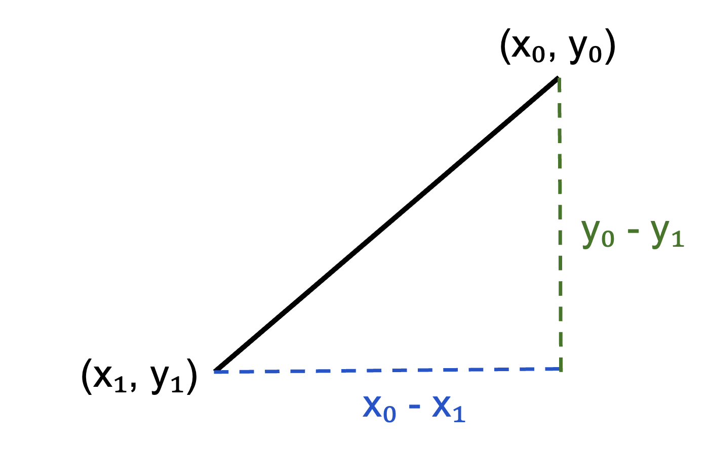
\[ D = \sqrt{(x_0-x_1)^2 + (y_0-y_1)^2}. \]

Distance Between Two Points

Two attributes x and y:

\[ D = \sqrt{(x_0-x_1)^2 + (y_0-y_1)^2}. \]

Three attributes x, y, z:

\[ D = \sqrt{(x_0-x_1)^2 + (y_0-y_1)^2 + (z_0-z_1)^2}. \]

and so on…

Distance Between Two Points in 2D

\[ D = \sqrt{(x_0-x_1)^2 + (y_0-y_1)^2}. \]

distance <- function(point1, point2) {
  # point1 and point2 are numeric vectors of the same length
  sqrt(sum((point1 - point2)^2))
}

Nearest Neighbors

Finding the \(k\) Nearest Neighbors

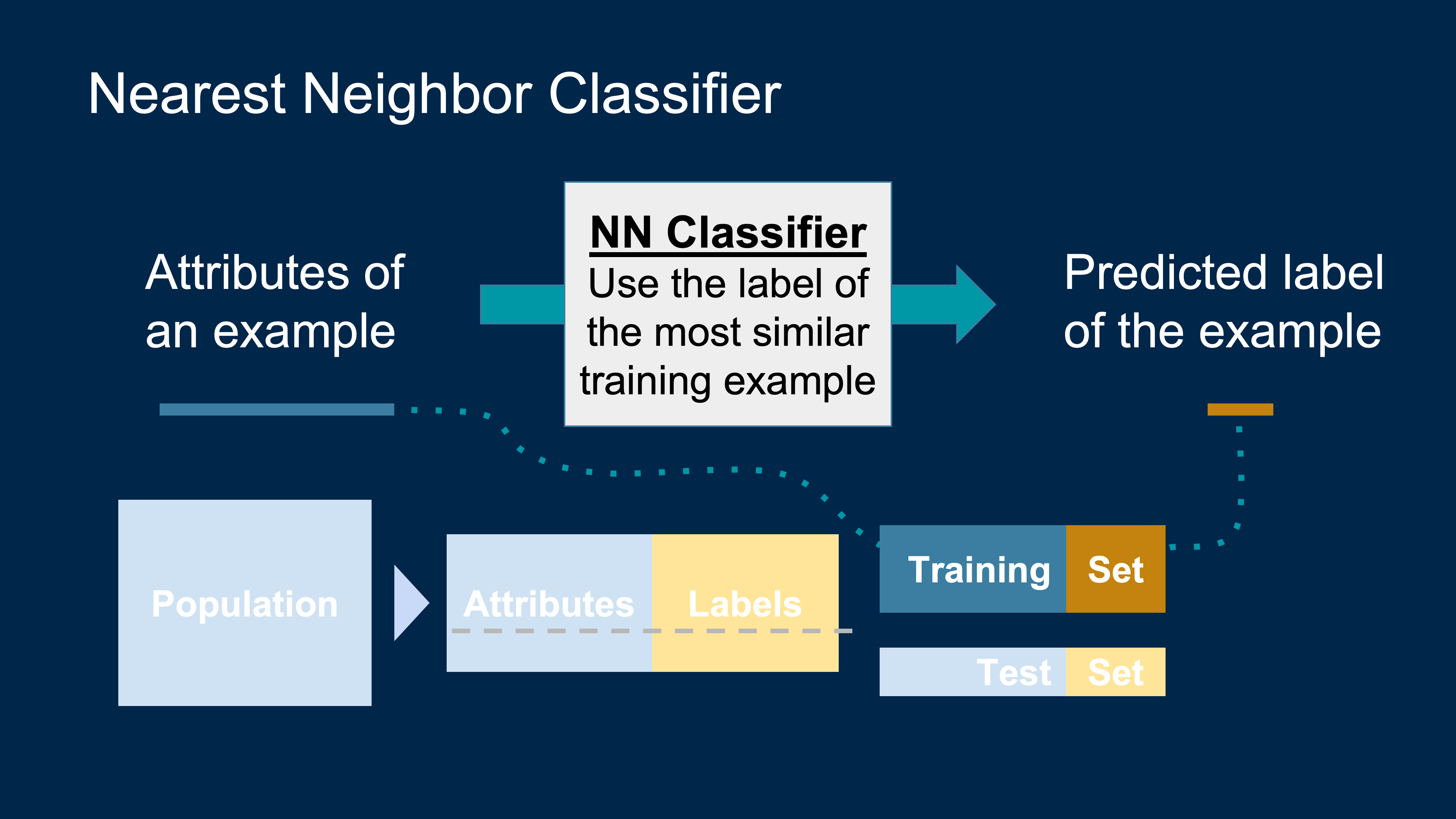
To find the k nearest neighbors of an example:

• Find the distance between the example and each example in the training set
• Augment the training data table with a column containing all the distances
• Sort the augmented table in increasing order of the distances
• Take the top k rows of the sorted table

The Classifier

To classify a point:

• Find its \(k\) nearest neighbors
• Take a majority vote of the \(k\) nearest neighbors to see which of the two classes appears more often
• Assign the point to the class that wins the majority vote

Wine Example: Data

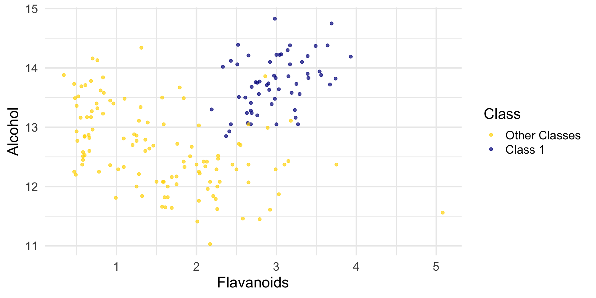
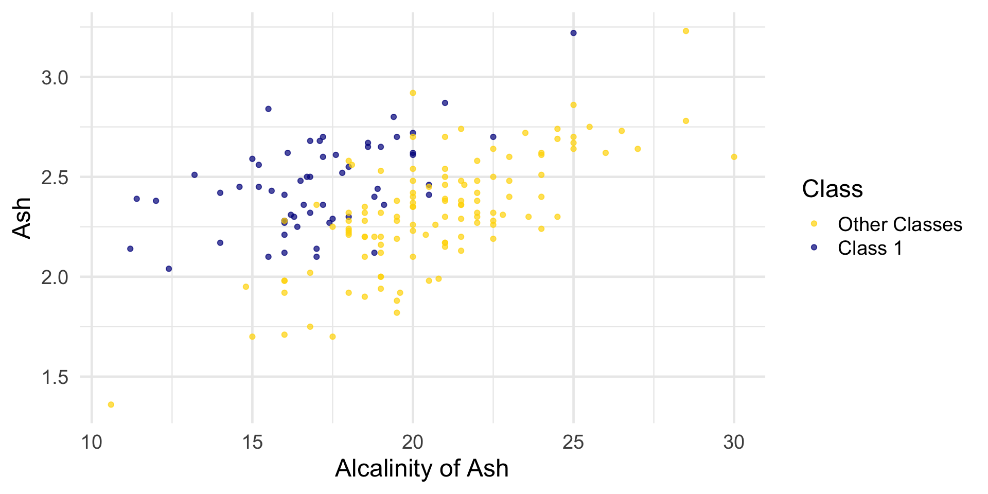
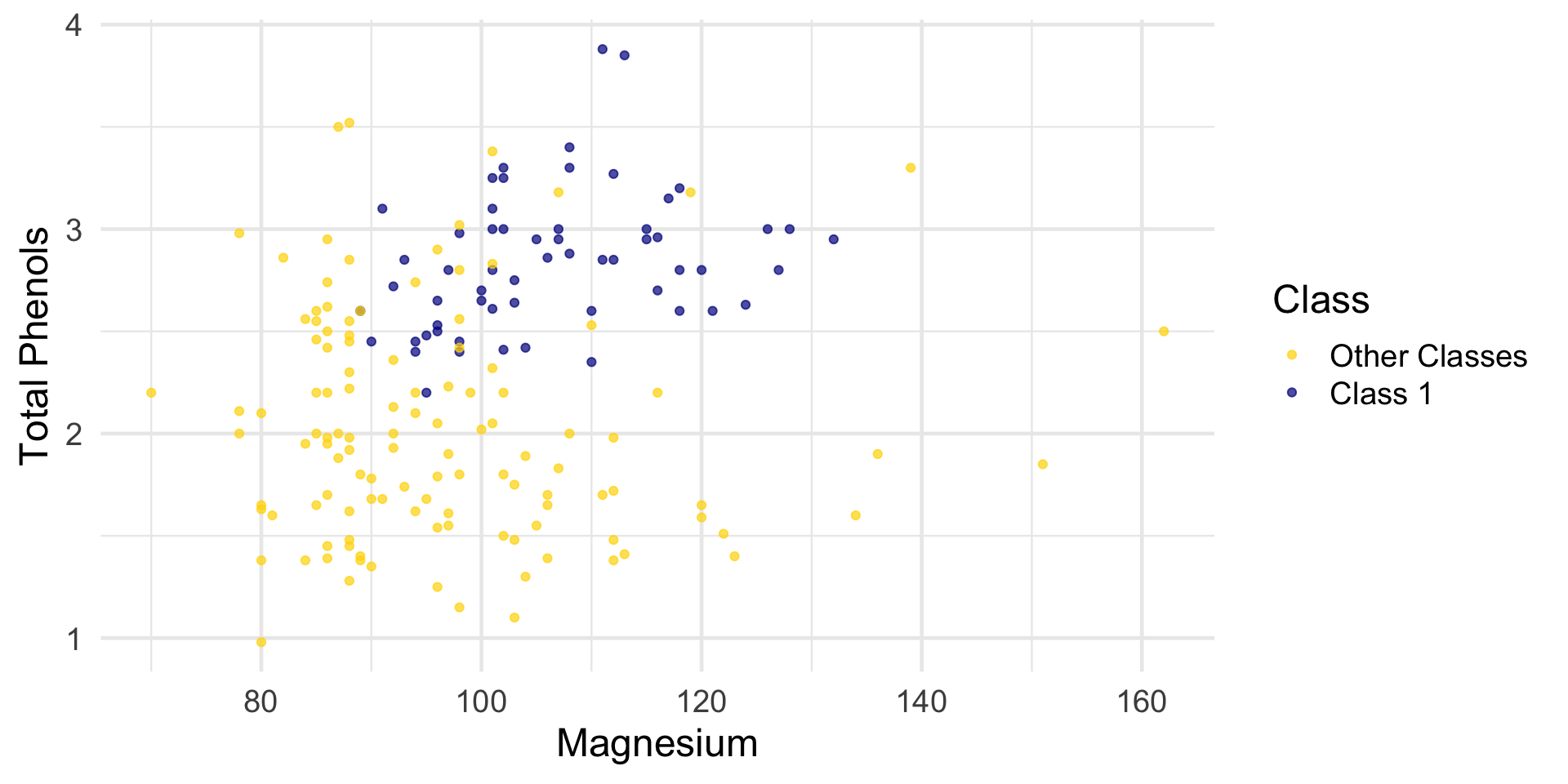
Read wine with three class. Classify Class 1 as level 1 and the other two classes as level 0.

wine <- read_csv("data/wine.csv") |>
  mutate(
    Class = factor(
      if_else(Class == 1, 1, 0),
      levels = c(0, 1),
      labels = c("Other Classes", "Class 1")
    )
  )

wine

# A tibble: 178 × 14
   Class   Alcohol `Malic Acid`   Ash `Alcalinity of Ash` Magnesium
   <fct>     <dbl>        <dbl> <dbl>               <dbl>     <dbl>
 1 Class 1    14.2         1.71  2.43                15.6       127
 2 Class 1    13.2         1.78  2.14                11.2       100
 3 Class 1    13.2         2.36  2.67                18.6       101
 4 Class 1    14.4         1.95  2.5                 16.8       113
 5 Class 1    13.2         2.59  2.87                21         118
 6 Class 1    14.2         1.76  2.45                15.2       112
 7 Class 1    14.4         1.87  2.45                14.6        96
 8 Class 1    14.1         2.15  2.61                17.6       121
 9 Class 1    14.8         1.64  2.17                14          97
10 Class 1    13.9         1.35  2.27                16          98
# ℹ 168 more rows
# ℹ 8 more variables: `Total Phenols` <dbl>, Flavanoids <dbl>,
#   `Nonflavanoid phenols` <dbl>, Proanthocyanins <dbl>,
#   `Color Intensity` <dbl>, Hue <dbl>, `OD280/OD315 of diulted wines` <dbl>,
#   Proline <dbl>

Wine Example: Distances

The first two wines are both in Class 1. To find the distance between them, we first need a data frame of just the attributes:

wine_attributes <- wine |>
  select(-Class) 

distance(wine_attributes[1, ], wine_attributes[2, ])

[1] 31.26501

distance(wine_attributes[1, ], wine_attributes[nrow(wine_attributes), ])

[1] 506.0594

That distance is quite a bit bigger!

Wine Example: Visualizing Classes

Wine Example: Visualizing Classes

Wine Example: Visualizing Classes

k-NN: Implementation Idea

Let’s see if we can implement a classifier based on all of the attributes.

The general approach is:

1. Find the closest \(k\) neighbors of point.
2. Look at the classes of those \(k\) neighbors and take the majority vote to find the most common class of wine.
   
3. Use that as our predicted class for point.

We’ll use the tidymodels framework to implement the classifier.

k-NN with tidymodels: Model Spec

Set up the model specification.

• We choose the k-nearest neighbors algorithm using the 5 nearest neighbors.
  
• We use the kknn engine (an implementation of k-NN).
  
• We set the mode to "classification" because we want to predict a class label.

knn_spec <- nearest_neighbor(neighbors = 5) |>
  set_engine("kknn") |>
  set_mode("classification")

k-NN with tidymodels: Fit on Wine Data

Next, we define how the model should learn from the data.

knn_fit <- knn_spec |>
  fit(Class ~ ., data = wine)

k-NN with tidymodels: Predict Wine Data

Now we can plug in a row of predictor values to make a prediction:

special_wine <- wine_attributes[1,]

predict(knn_fit, new_data = special_wine)

# A tibble: 1 × 1
  .pred_class
  <fct>      
1 Class 1    

k-NN with tidymodels: Predict Wine Data

What about something from Other Classes?

special_wine <- wine_attributes[nrow(wine),]

predict(knn_fit, new_data = special_wine)

# A tibble: 1 × 1
  .pred_class  
  <fct>        
1 Other Classes

Yes! The classifier gets this one right too.

But we don’t yet know how it does with all the other wines. Also, testing on wines that are already part of the training set might be over-optimistic.

Hold-Out Method

To get an unbiased estimate of our classifier’s accuracy, we split the data into:

• a training set (used to fit the model), and
  
• a test set (held out until the end, to evaluate accuracy).

This is sometimes called the hold-out method.

Hold-Out Method

We’ll randomly split the 178 wines into 89 training and 89 test examples.

data_split <- initial_split(wine, prop = 0.505, strata = Class)
train_data <- training(data_split)
test_data  <- testing(data_split)

nrow(train_data); nrow(test_data)

[1] 89

[1] 89

Measuring Wine Classifier Accuracy

First, we set up and train the classifier on train_data:

knn_spec <- nearest_neighbor(neighbors = 5) |>
  set_engine("kknn") |>
  set_mode("classification")

knn_fit <- knn_spec |>
  fit(Class ~ ., data = train_data)

Measuring Wine Classifier Accuracy

Then we get predictions on the test set:

knn_preds <- predict(knn_fit, new_data = test_data)

knn_preds

# A tibble: 89 × 1
   .pred_class
   <fct>      
 1 Class 1    
 2 Class 1    
 3 Class 1    
 4 Class 1    
 5 Class 1    
 6 Class 1    
 7 Class 1    
 8 Class 1    
 9 Class 1    
10 Class 1    
# ℹ 79 more rows

Measuring Wine Classifier Accuracy

The last step is to compare how many of these predictions are correct by looking at the true labels from test_data:

test_data |>
  mutate(predicted = knn_preds$.pred_class) |>
  accuracy(truth = Class, estimate = predicted)

# A tibble: 1 × 3
  .metric  .estimator .estimate
  <chr>    <chr>          <dbl>
1 accuracy binary         0.989

The accuracy rate isn’t bad at all for a simple classifier!

Breast Cancer: Train/Test Split

The data set has 683 patients. We’ll randomly permute the dataset and put 342 in the training set and the remaining 341 in the test set.

data_split <- initial_split(patients, prop = 343/683, strata = Class)
train_data <- training(data_split)
test_data  <- testing(data_split)

nrow(train_data); nrow(test_data)

[1] 342

[1] 341

Breast Cancer: k-NN Classifier

Let’s stick with 5 nearest neighbors, and see how well our classifier does.

knn_spec <- nearest_neighbor(neighbors = 5) |>
  set_engine("kknn") |>
  set_mode("classification")

knn_fit <- knn_spec |>
  fit(Class ~ ., data = train_data)

knn_preds <- predict(knn_fit, new_data = test_data)

head(knn_preds)

# A tibble: 6 × 1
  .pred_class
  <fct>      
1 benign     
2 benign     
3 benign     
4 malignant  
5 benign     
6 benign     

Breast Cancer: Accuracy

Now compare predictions to the true labels to measure accuracy:

test_data |>
  mutate(predicted = knn_preds$.pred_class) |>
  accuracy(truth = Class, estimate = predicted)

# A tibble: 1 × 3
  .metric  .estimator .estimate
  <chr>    <chr>          <dbl>
1 accuracy binary         0.974

Before Classifying

Visualize your features

Banknotes Demo

Start with a Representative Sample

• Both the training and test sets must accurately represent the population on which you use your classifier
• Overfitting happens when a classifier does very well on the training set, but can’t do as well on the test set

Standardize if Necessary

• If the attributes are on very different numerical scales, distance can be affected
• In such a situation, it is a good idea to convert all the variables to standard units

Example: CKD

standard_units <- function(x){
  (x - mean(x))/sd(x)
}

ckd <- read_csv('data/ckd.csv') |> 
  rename(Glucose = `Blood Glucose Random`) |>
  mutate(
    Hemoglobin = standard_units(Hemoglobin),
    Glucose = standard_units(Glucose),
    `White Blood Cell Count` = standard_units(`White Blood Cell Count`),
    Class = factor(Class,
                   levels = c(0, 1),
                   labels = c("No CKD", "CKD")) 
  ) |>
  select(Hemoglobin, Glucose, `White Blood Cell Count`, Class)

Example: CKD

data_split <- initial_split(patients, prop = 75/148, strata = Class)
train_data <- training(data_split)
test_data  <- testing(data_split)


knn_spec <- nearest_neighbor(neighbors = 5) |>
  set_engine("kknn") |>
  set_mode("classification")

knn_fit <- knn_spec |>
  fit(Class ~ ., data = train_data)

knn_preds <- predict(knn_fit, new_data = test_data)

test_data |>
  mutate(predicted = knn_preds$.pred_class) |>
  accuracy(truth = Class, estimate = predicted)

# A tibble: 1 × 3
  .metric  .estimator .estimate
  <chr>    <chr>          <dbl>
1 accuracy binary         0.979

Workflow for Supervised Learning

1. Define the task
   • What are we predicting? (numeric \(Y\) or categorical \(Y\)?)
   • What are the features \(X\) available?
2. Prepare the data
   • Clean, handle missing values.
   • Encode categorical variables (e.g., one-hot encoding).
3. Split the data
   • Training set vs test set.
4. Choose a model
   • Regression line, \(k\)-nearest neighbors, etc.
5. Train the model
   • Fit the model on the training data.
6. Evaluate on test data
   • Regression: RMSE, \(R^2\), etc.
   • Classification: accuracy, sensitivity, etc.