Data Frame in R

Sarah Cassie Burnett

September 4, 2025

Before we get started…

Check your version of the tidyverse library in the Console:

packageVersion("tidyverse")

[1] '2.0.0'

or install it during lecture:

install.packages("tidyverse")

Scan and fill out for participation credit

https://forms.gle/neFgQu8wcrbWXGQ9A

Annoucements

Quiz today.
Next in class quiz on Thursday.
Coding Assignment 1 to be posted today to be due next Thursday 11:59 pm.

Scan and fill out for participation credit

https://forms.gle/neFgQu8wcrbWXGQ9A

Some Common Base R Functions

Aggregate functions

(these take a whole vector and return a single summary value)

mean() mean of a set of numbers
median() median of a set of numbers
sd() standard deviation of a set of numbers
sum() sum of a set of numbers
length() length of a vector
max() / min() maximum and minimum values of a vector

Some Common Base R Functions

Elementwise functions

(these apply a transformation to each element of a vector)

round() round to a specified number of decimal places
sqrt() square root
log() natural logarithm
exp() exponential
abs() absolute value

Indexing in R

Use indexing to extract a subset of your container
You can access elements of a vector in several ways:
- By position
- By negative index
- By boolean/logical expressions
- By name

Packages

From Functions to Packages

A function is a set of instructions
- read_csv() is a function
- sample() is a function
A package is a collection of functions
- readr is a package that contains the read_csv() function
- ggplot2 is a package that contains the ggplot() function
Use install.packages() to install packages
Use library() to load packages
You can install packages from CRAN

A Data Science Workflow

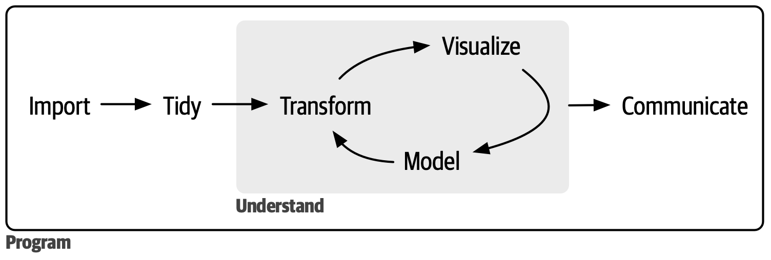
The Tidyverse

The Tidyverse is a collection of data science packages
It is also considered a dialect of R
In this class, we will be using many Tidyverse packages
- readr for reading data
- tidyr for data tidying
- dplyr for data manipulation
- ggplot2 for data visualization
Click here for a full list

Working with Tidyverse packages

At first we will load the packages independently, e.g. library(ggplot2)
Later we will load them all at once with library(tidyverse)
Another way to call a package is with ::, e.g. ggplot2::ggplot()

Dataframe

What is this?

name <- c("Cars", "WALL-E", "The Lego Movie", "PAW Patrol: The Movie")
lead_person <- c("Lightning McQueen (Owen Wilson)",
                 "WALL-E (Ben Burtt)",
                 "Emmet Brickowski (Chris Pratt)",
                 "Ryder (Will Brisbin)")
length_minutes <- c(120, 97, 101, 86)
award <- c(TRUE, TRUE, TRUE, FALSE)

df <- data.frame(
  name,
  lead_person,
  length_minutes,
  award
)

Reading Data into R

Download some data: Download the ZIP version
Let’s use the readr package to read in a dataset

library(readr)

films <- read_csv2("data/film.csv")
# or
films <- read_csv("data/film_cleanish.csv")

Let’s Look at the Data

One way to do this is with the base R head() function

head(films)

# A tibble: 6 × 9
   Year Length Title    Genre `Lead Man` `Lead Woman` Director Popularity Awards
  <dbl>  <dbl> <chr>    <chr> <chr>      <chr>        <chr>         <dbl> <lgl> 
1  1990    111 Tie Me … Come… Banderas,… Abril, Vict… Almodóv…         68 FALSE 
2  1991    113 High He… Come… Bosé, Mig… Abril, Vict… Almodóv…         68 FALSE 
3  1983    104 Dead Zo… Horr… Walken, C… Adams, Broo… Cronenb…         79 FALSE 
4  1979    122 Cuba     Acti… Connery, … Adams, Broo… Lester,…          6 FALSE 
5  1978     94 Days of… Drama Gere, Ric… Adams, Broo… Malick,…         14 FALSE 
6  1983    140 Octopus… Acti… Moore, Ro… Adams, Maud  Glen, J…         68 FALSE

Use `View()`

Another way to look at the data is with View(). Or click on the name of the data frame in the Environment pane.

View(films)

Using `glimpse()` from `dplyr`

Another way to look at the data is with glimpse() from the dplyr package.

library(dplyr)

glimpse(films)

Rows: 1,659
Columns: 9
$ Year         <dbl> 1990, 1991, 1983, 1979, 1978, 1983, 1984, 1989, 1985, 199…
$ Length       <dbl> 111, 113, 104, 122, 94, 140, 101, 99, 104, 149, 188, 117,…
$ Title        <chr> "Tie Me Up! Tie Me Down!", "High Heels", "Dead Zone, The"…
$ Genre        <chr> "Comedy", "Comedy", "Horror", "Action", "Drama", "Action"…
$ `Lead Man`   <chr> "Banderas, Antonio", "Bosé, Miguel", "Walken, Christopher…
$ `Lead Woman` <chr> "Abril, Victoria", "Abril, Victoria", "Adams, Brooke", "A…
$ Director     <chr> "Almodóvar, Pedro", "Almodóvar, Pedro", "Cronenberg, Davi…
$ Popularity   <dbl> 68, 68, 79, 6, 14, 68, 14, 28, 6, 32, 81, 17, 46, 49, 6, …
$ Awards       <lgl> FALSE, FALSE, FALSE, FALSE, FALSE, FALSE, FALSE, FALSE, F…

Try it out!

Read in the film_cleanish.csv file
Use the three methods we discussed to view the data

05:00

A Few More Basic `dplyr` Functions

Use select() to choose columns.

films_select <- films |>
     select(Title, Awards)

glimpse(films_select)

Rows: 1,659
Columns: 2
$ Title  <chr> "Tie Me Up! Tie Me Down!", "High Heels", "Dead Zone, The", "Cub…
$ Awards <lgl> FALSE, FALSE, FALSE, FALSE, FALSE, FALSE, FALSE, FALSE, FALSE, …

A Few More Basic `dplyr` Functions

Use filter() to choose rows.

films <- read_csv("data/film_cleanish.csv")

films_select <- films |>
  filter(Awards == TRUE)

# or
films_select <- films |>
  filter(Awards)

Note

Using the same name for the data frame results in overwriting the original data frame. If you want to keep the original data frame, use a different name.

A Few More Basic `dplyr` Functions

Use mutate() to create new columns.

films_new <- films |>
  mutate(Length_hours = Length / 60)

glimpse(films_new)

Rows: 1,659
Columns: 10
$ Year         <dbl> 1990, 1991, 1983, 1979, 1978, 1983, 1984, 1989, 1985, 199…
$ Length       <dbl> 111, 113, 104, 122, 94, 140, 101, 99, 104, 149, 188, 117,…
$ Title        <chr> "Tie Me Up! Tie Me Down!", "High Heels", "Dead Zone, The"…
$ Genre        <chr> "Comedy", "Comedy", "Horror", "Action", "Drama", "Action"…
$ `Lead Man`   <chr> "Banderas, Antonio", "Bosé, Miguel", "Walken, Christopher…
$ `Lead Woman` <chr> "Abril, Victoria", "Abril, Victoria", "Adams, Brooke", "A…
$ Director     <chr> "Almodóvar, Pedro", "Almodóvar, Pedro", "Cronenberg, Davi…
$ Popularity   <dbl> 68, 68, 79, 6, 14, 68, 14, 28, 6, 32, 81, 17, 46, 49, 6, …
$ Awards       <lgl> FALSE, FALSE, FALSE, FALSE, FALSE, FALSE, FALSE, FALSE, F…
$ Length_hours <dbl> 1.850000, 1.883333, 1.733333, 2.033333, 1.566667, 2.33333…

Try it out!

Use your new dplyr verbs to manipulate the data
Select columns, filter rows, and create new columns

05:00

Basic Data Viz with `ggplot2`

ggplot2 is a powerful data visualization package
It is based on the grammar of graphics
We will talk about this more in depth later

Basic Data Viz with `ggplot2`

For now, let’s make a simple column chart

Code

library(ggplot2)

ggplot(data = films, aes(x = Genre, y = Popularity)) +
  geom_col(fill = "dodgerblue")

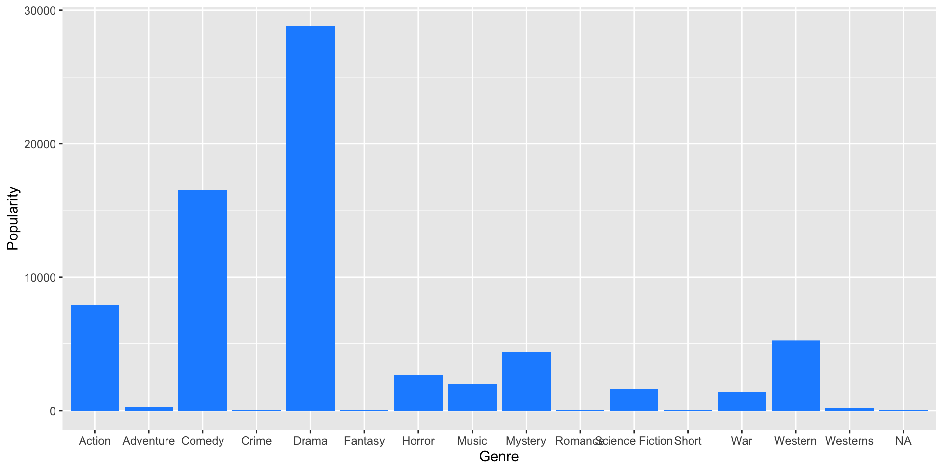
Try it out!

Use ggplot2 to make a simple column chart
Choose a different variable to plot
Change the color of the bars

05:00

Data Frame in R

Before we get started…

Annoucements

Some Common Base R Functions

Aggregate functions

Some Common Base R Functions

Elementwise functions

Indexing in R

Packages

From Functions to Packages

A Data Science Workflow

The Tidyverse

Working with Tidyverse packages

Dataframe

Reading Data into R

Let’s Look at the Data

Use View()

Using glimpse() from dplyr

Try it out!

A Few More Basic dplyr Functions

A Few More Basic dplyr Functions

A Few More Basic dplyr Functions

Try it out!

Basic Data Viz with ggplot2

Basic Data Viz with ggplot2

Try it out!

Use `View()`

Using `glimpse()` from `dplyr`

A Few More Basic `dplyr` Functions

A Few More Basic `dplyr` Functions

A Few More Basic `dplyr` Functions

Basic Data Viz with `ggplot2`

Basic Data Viz with `ggplot2`