Categorical vs. Continuous Data

Sarah Cassie Burnett

October 7, 2025

Today

• What do we mean by categorical vs continuous?
• Why types matter for summaries and visuals

What are some ways we can classify data?

• anecdotal vs. representative
• census vs. sample
• observational vs. experimental
• categorical vs. numerical
• discrete vs. continuous
• cross-sectional vs. time series
• longitudinal vs. panel
• unstructured vs. structured

What are some ways we can classify data?

• anecdotal vs. representative
• census vs. sample
• observational vs. experimental
• categorical vs. numerical
• discrete vs. continuous
• cross-sectional vs. time series
• longitudinal vs. panel
• unstructured vs. structured

Variable Types

• Categorical

  • Binary - two categories
  • Nominal - multiple unordered categories
  • Ordinal - multiple ordered categories

• Numerical

  • Continuous - a range of numbers (measurement data)
  • Discrete - take on separate, distinct values (countable data)

Create a (random) daily-life dataset

library(tidyverse) # let's load in everything
set.seed(7) # we are going to create something random
            # the 'seed' is so my random looks like your random

N <- 60 #number of observations

lifelog <- tibble(
  id = 1:N,                                    # identifier (categorical by meaning)
  age = sample(18:35, N, replace = TRUE),      # numeric (discrete integer)
  height_cm = round(rnorm(N, mean = 170, sd = 10), 1),  # continuous
  commute_mode = sample(c("Walk","Bike","Transit","Car"), N, replace = TRUE), # categorical (nominal)
  coffee_cups = sample(0:5, N, replace = TRUE),      # counts (discrete numeric)
  coffee_today = coffee_cups > 0,               # logical/binary (categorical by meaning)
  study_hours = round(runif(N, 0, 6), 1),      # continuous
  mood = factor(sample(c("Low","Medium","High"), N, replace = TRUE),
                levels = c("Low","Medium","High"), ordered = TRUE), # categorical (ordinal)
  zip_code = sample(c("20001","20002","20037","20052"), N, replace = TRUE) # numeric-looking categorical
)

The Two Big Families

Family	Meaning	R classes you’ll see	Typical summaries	Typical visuals
Categorical	labels/groups (nominal or ordered)	factor, ordered, character, logical	counts, proportions	bar charts, stacked bars
Continuous	measurements in a range	numeric, double, integer	mean/median, sd/IQR, quantiles	histogram, line plot, scatterplot, boxplot

Categorical Data

Classify

What counts as categorical?

• Nominal: commute_mode, zip_code
  
• Ordinal: mood (Low < Medium < High)
  
• Binary: coffee_today (TRUE/FALSE)

Summarize one categorical variable

# counts & proportions
lifelog |>
  count(commute_mode) |>
  mutate(prop = n / sum(n)) |>
  arrange(desc(n))

# A tibble: 4 × 3
  commute_mode     n  prop
  <chr>        <int> <dbl>
1 Car             17 0.283
2 Walk            17 0.283
3 Transit         15 0.25 
4 Bike            11 0.183

Visualize

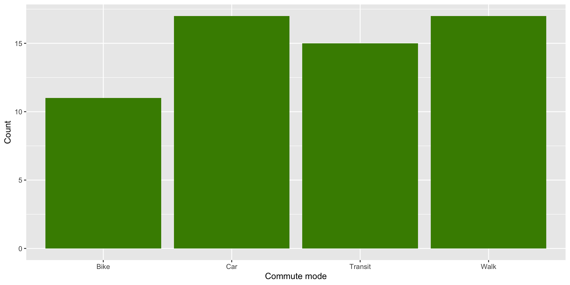
Single categorical variable: use bar chart

ggplot(lifelog, aes(x = commute_mode)) +
  geom_bar(fill="chartreuse4") +
  labs(x = "Commute mode", y = "Count")

Visualize

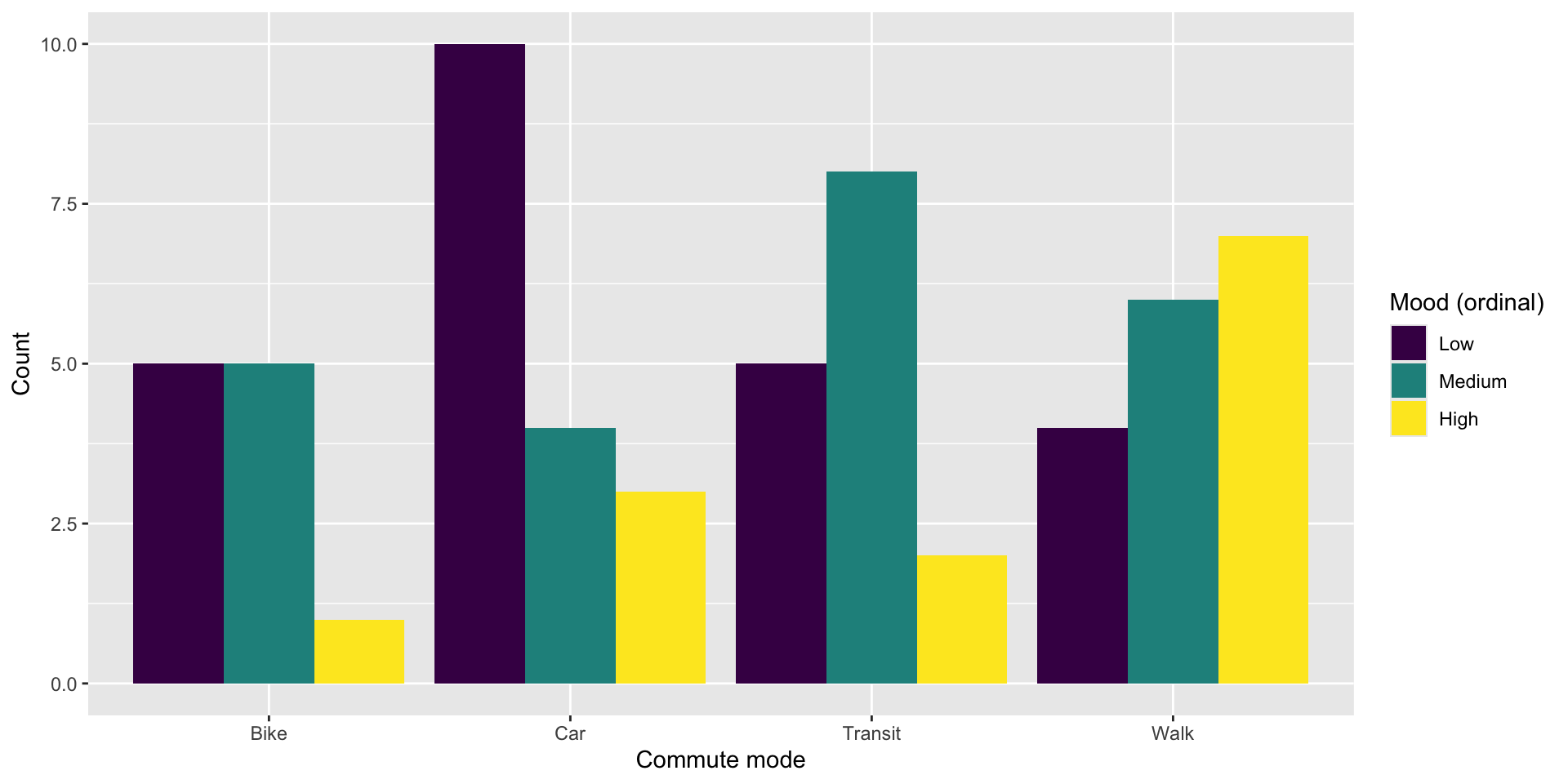
Two categorical variables: dodged bars

ggplot(lifelog, aes(x = commute_mode, fill = mood)) +
  geom_bar(position = "dodge") +
  labs(x = "Commute mode", y = "Count", fill = "Mood (ordinal)")

Visualize

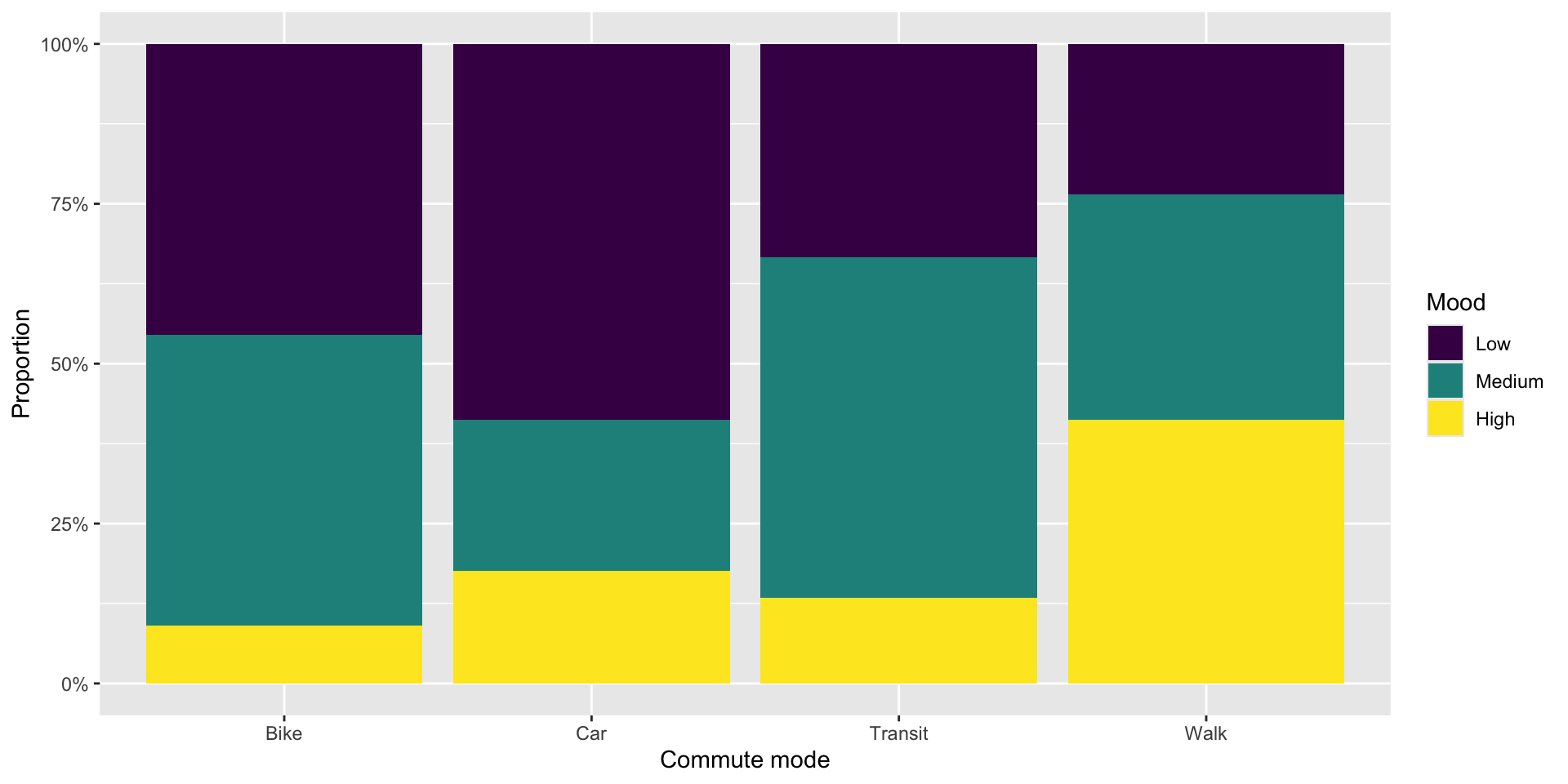
Two categorical variables: stacked bars

ggplot(lifelog, aes(x = commute_mode, fill = mood)) +
  geom_bar(position = "fill") +
  scale_y_continuous(labels = scales::percent) +
  labs(x = "Commute mode", y = "Proportion", fill = "Mood")

Continuous Data

Classify

What counts as continuous?

• Measurements: height_cm, study_hours
• Counts (discrete numeric): coffee_cups (treated similarly but integer-valued)

Summarize

lifelog |>
  summarize(
    mean_height   = mean(height_cm),
    sd_height     = sd(height_cm),
    median_height = median(height_cm),
    q25_height    = quantile(height_cm, 0.25),
    q75_height    = quantile(height_cm, 0.75),
    mean_study    = mean(study_hours),
    sd_study      = sd(study_hours),
    median_study  = median(study_hours),
    q25_study     = quantile(study_hours, 0.25),
    q75_study     = quantile(study_hours, 0.75)
  )

# A tibble: 1 × 10
  mean_height sd_height median_height q25_height q75_height mean_study sd_study
        <dbl>     <dbl>         <dbl>      <dbl>      <dbl>      <dbl>    <dbl>
1        172.      8.19           174       167.       178.       2.93     1.81
# ℹ 3 more variables: median_study <dbl>, q25_study <dbl>, q75_study <dbl>

Visualize

One continuous variable: histogram

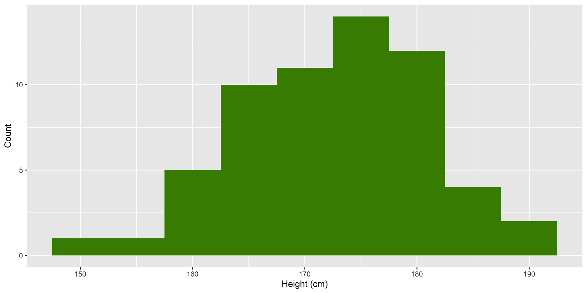
# histogram
ggplot(lifelog, aes(x = height_cm)) +
  geom_histogram(binwidth = 5, fill="chartreuse4") +
  labs(x = "Height (cm)", y = "Count") 

Visualize

Two continuous variables: scatterplots

ggplot(lifelog, aes(x = height_cm, y = study_hours)) +
  geom_point(color = "darkorange", alpha = 0.7) +
  labs(x = "Height (cm)", y = "Study hours (per day)") 

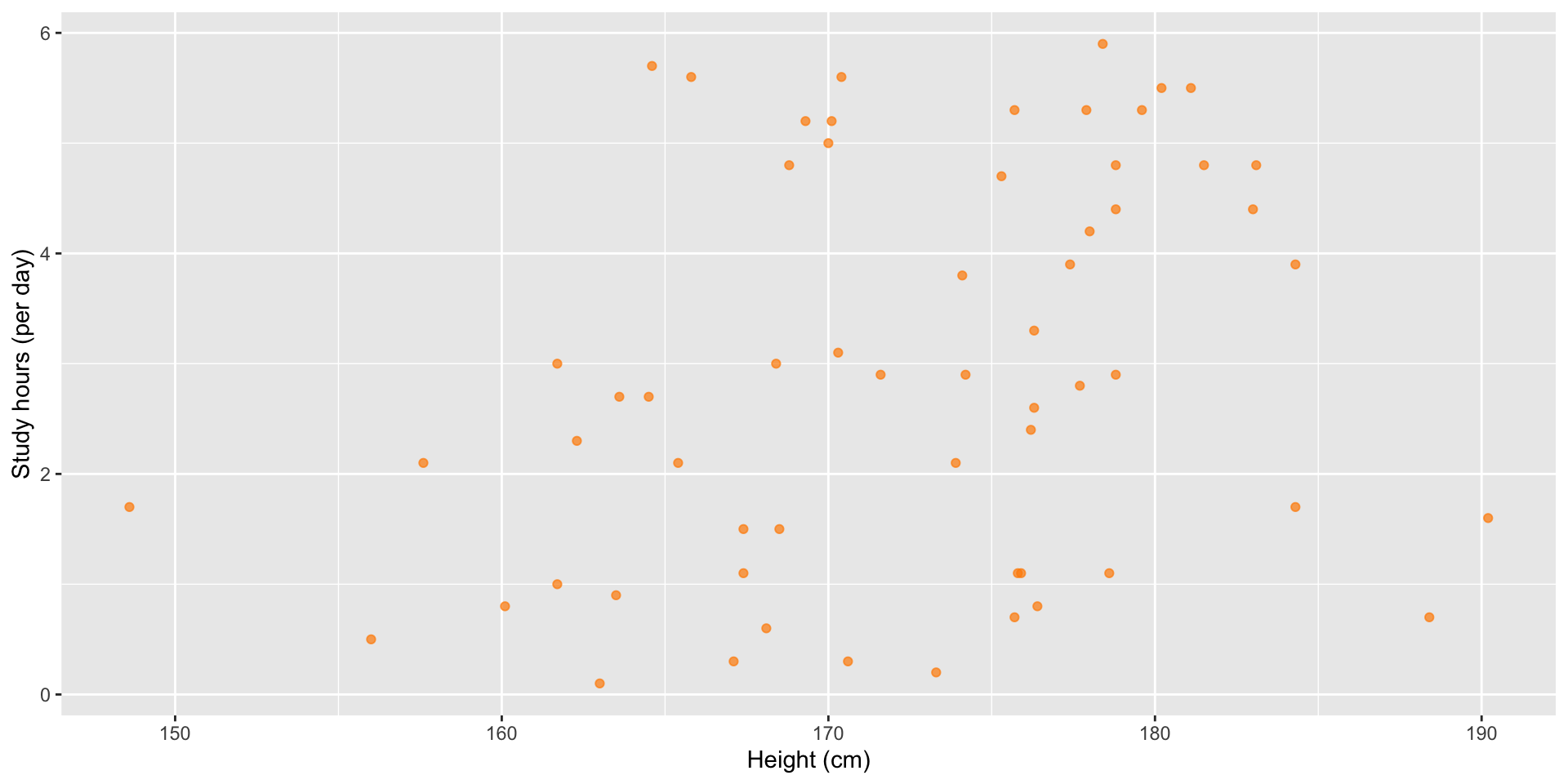
If one variable was time, a line chart would be recommended here.

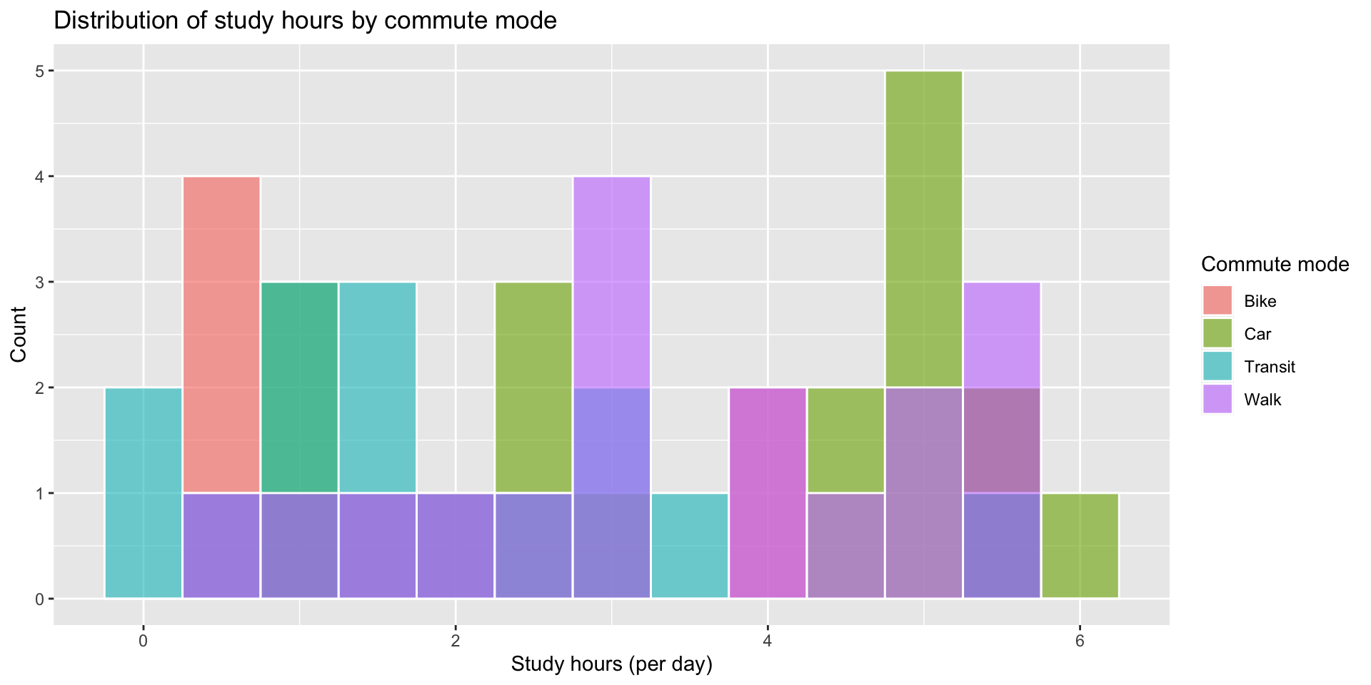
Visualize

What if you want to visualize continuous distributions across different categories?

Visualize

Histogram of continuous variable by category (not easy to see)

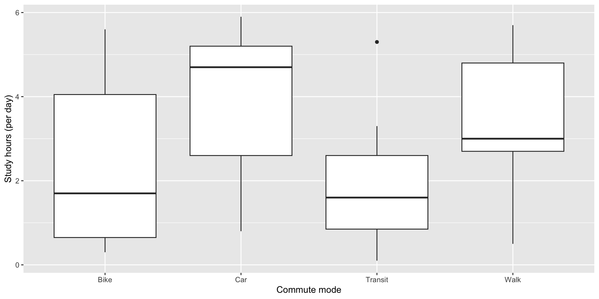
ggplot(lifelog, aes(x = study_hours, fill = commute_mode)) +
  geom_histogram(binwidth = 0.5, alpha = 0.6, position = "identity", color = "white") +
  labs(
    x = "Study hours (per day)",
    y = "Count",
    fill = "Commute mode",
    title = "Distribution of study hours by commute mode"
  )

Visualize

Boxplot of continuous by categorical

ggplot(lifelog, aes(x = commute_mode, y = study_hours)) +
  geom_boxplot() +
  labs(x = "Commute mode", y = "Study hours (per day)") 

Try it out!

Best visualization for each:
- height_cm → ?
- study_hours → ?
- coffee_cups (discrete count) → ?

Classify: continuous or categorical (nominal, ordinal, binary)
- coffee_today → ?
- mood → ?
- id, zip_code → ?

Summarize:
- Categorical → ?
- Continuous → ?

05:00

Try it out!

Best visualization for each:
- height_cm → histogram, boxplot - study_hours → histogram, boxplot - coffee_cups (discrete count) → histogram, boxplot

Classify: continuous or categorical (nominal, ordinal, binary)
- coffee_today → binary categorical
- mood → ordinal categorical
- id, zip_code → categorical identifiers

Summarize:
- Categorical → counts, proportions
- Continuous → mean/median, SD/IQR, quantiles

Other practices (continuous)

• Don’t take means of numerics used as labels like IDs or ZIP codes
  
• Check for outliers

# quick outlier peek for height
lifelog |>
  summarize(q05 = quantile(height_cm, .05), q95 = quantile(height_cm, .95))

# A tibble: 1 × 2
    q05   q95
  <dbl> <dbl>
1  160.  184.

Other practices (categorical)

• Unseen levels: set factor levels explicitly for consistent ordering

Factor vs. vector of characters

tbl <- tibble(month = c("March", "January", "February"))

# Default: character columns arrange alphabetically
tbl |> arrange(month)

# A tibble: 3 × 1
  month   
  <chr>   
1 February
2 January 
3 March   

tbl <- tbl |>
  mutate(month = factor(month, levels = c("January", "February", "March")))

# Now arrange() follows factor levels
tbl |> arrange(month)

# A tibble: 3 × 1
  month   
  <fct>   
1 January 
2 February
3 March