Measuring Distributions
Sarah Cassie Burnett
October 16, 2025
Undersampled vs. Well-sampled
Let’s look at penguin flipper length.
Here’s a histogram across three species:
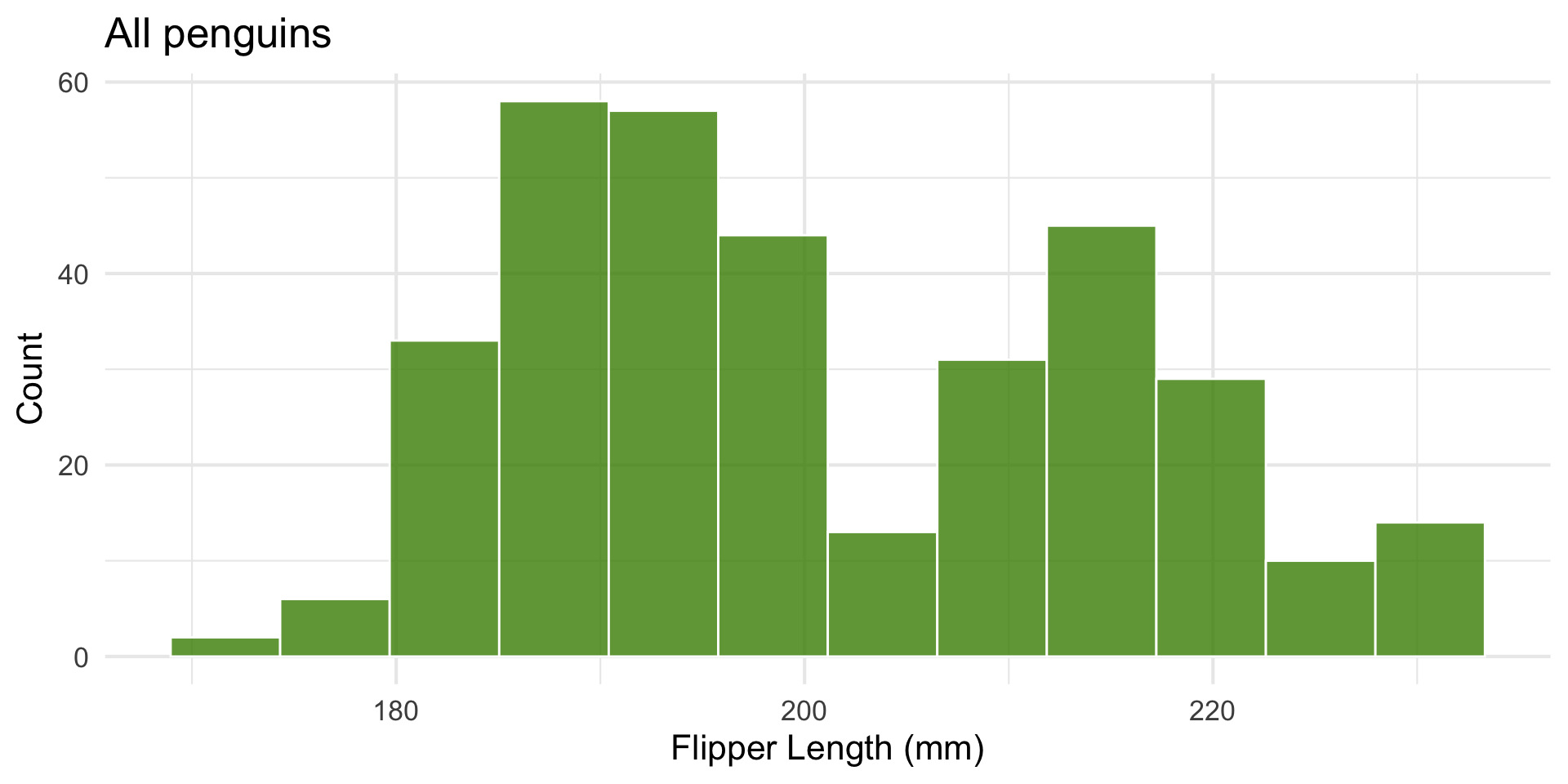
Look at one group’s distribution
Let’s look at penguin flipper length.
Filter for only ‘Adelie’.
Code
library(tidyverse)
library(palmerpenguins)
set.seed(7)

Adelie_penguins <- penguins |> filter(species == "Adelie")

ggplot(Adelie_penguins, aes(x = flipper_length_mm)) +
  geom_histogram(fill = "chartreuse4", color = "white", bins = 12, alpha = 0.8) +
  labs(
    title = "151 Adelie penguins",
    x = "Flipper Length (mm)",
    y = "Count") + theme_minimal(base_size = 16)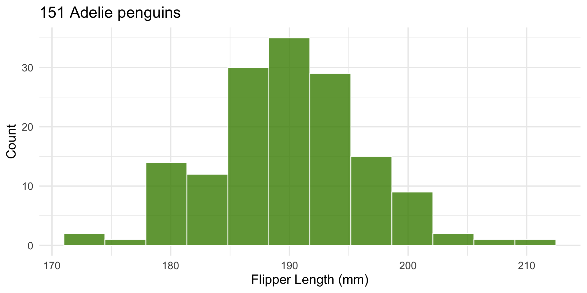
Undersampled vs. Well-sampled
Let’s look at penguin flipper length.
We’ll compare a tiny random sample to a large one.
Code
# Plot side by side
p_small <- ggplot(small_sample, aes(x = flipper_length_mm)) +
  geom_histogram(fill = "chartreuse4", color = "white", bins = 8, alpha = 0.8) +
  labs(
    title = "Undersampled (n = 10)",
    x = "Flipper Length (mm)",
    y = "Count"
  ) +
  theme_minimal(base_size = 16)

p_large <- ggplot(Adelie_penguins, aes(x = flipper_length_mm)) +
  geom_histogram(fill = "chartreuse4", color = "white", bins = 12, alpha = 0.8) +
  labs(
    title = "151 Adelie penguins",
    x = "Flipper Length (mm)",
    y = "Count"
  ) +
  theme_minimal(base_size = 16)

# Combine later with patchwork:
library(patchwork)
p_small + p_large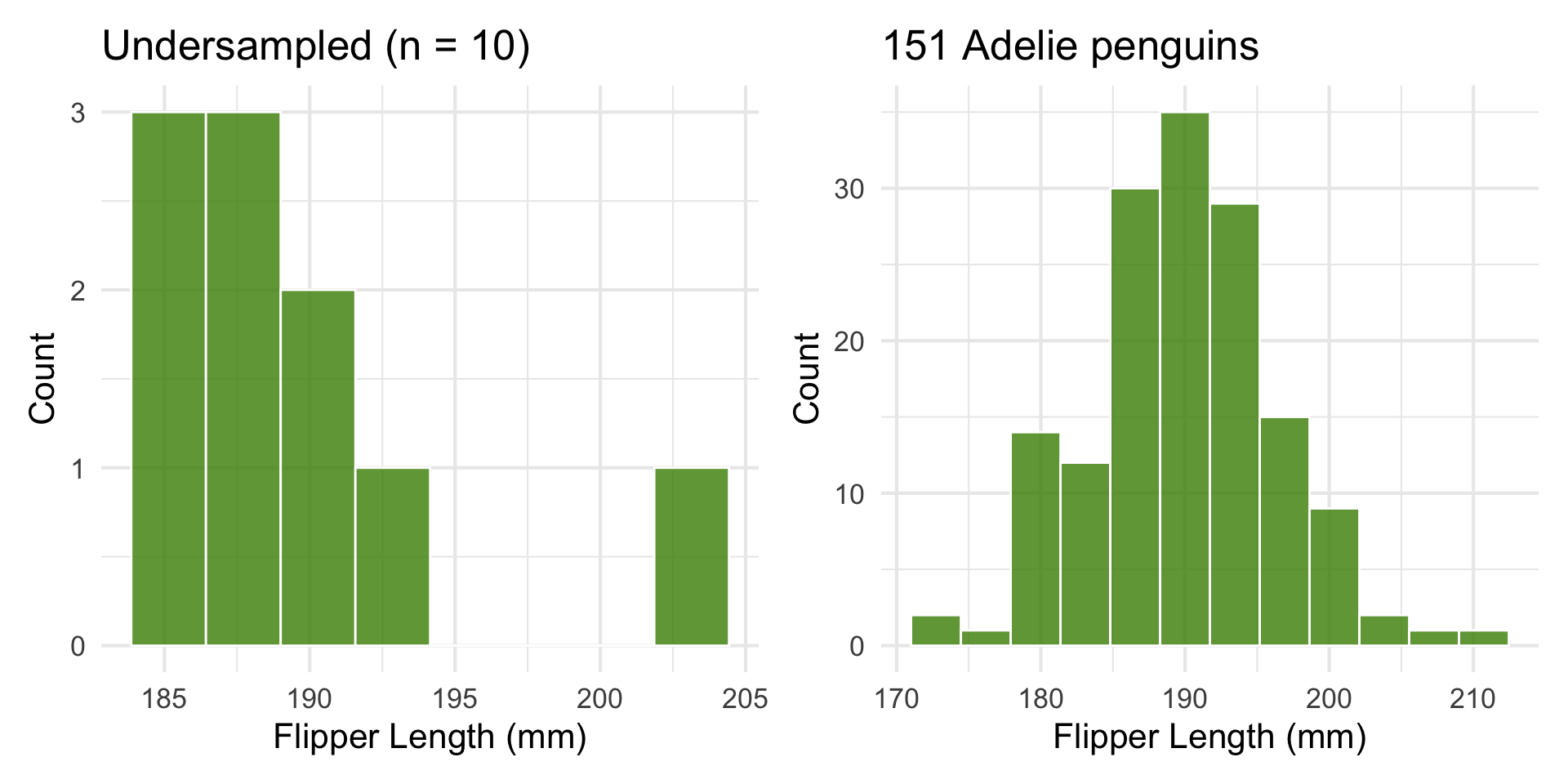
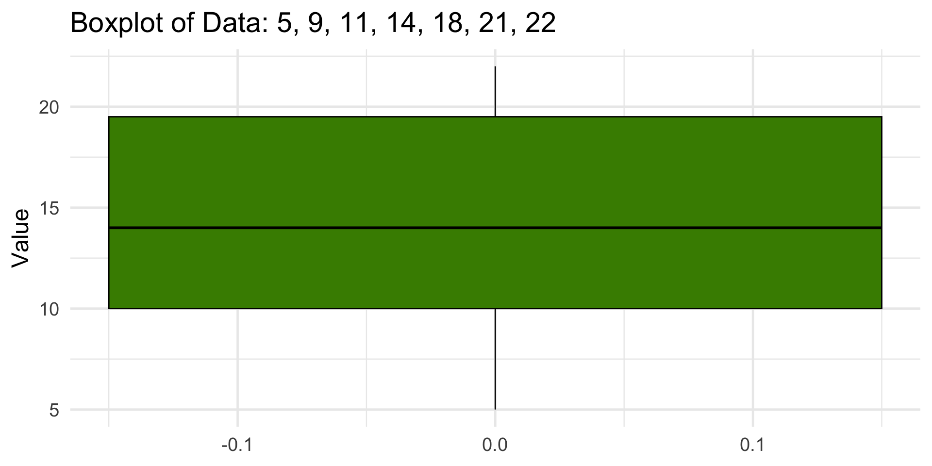
Boxplot
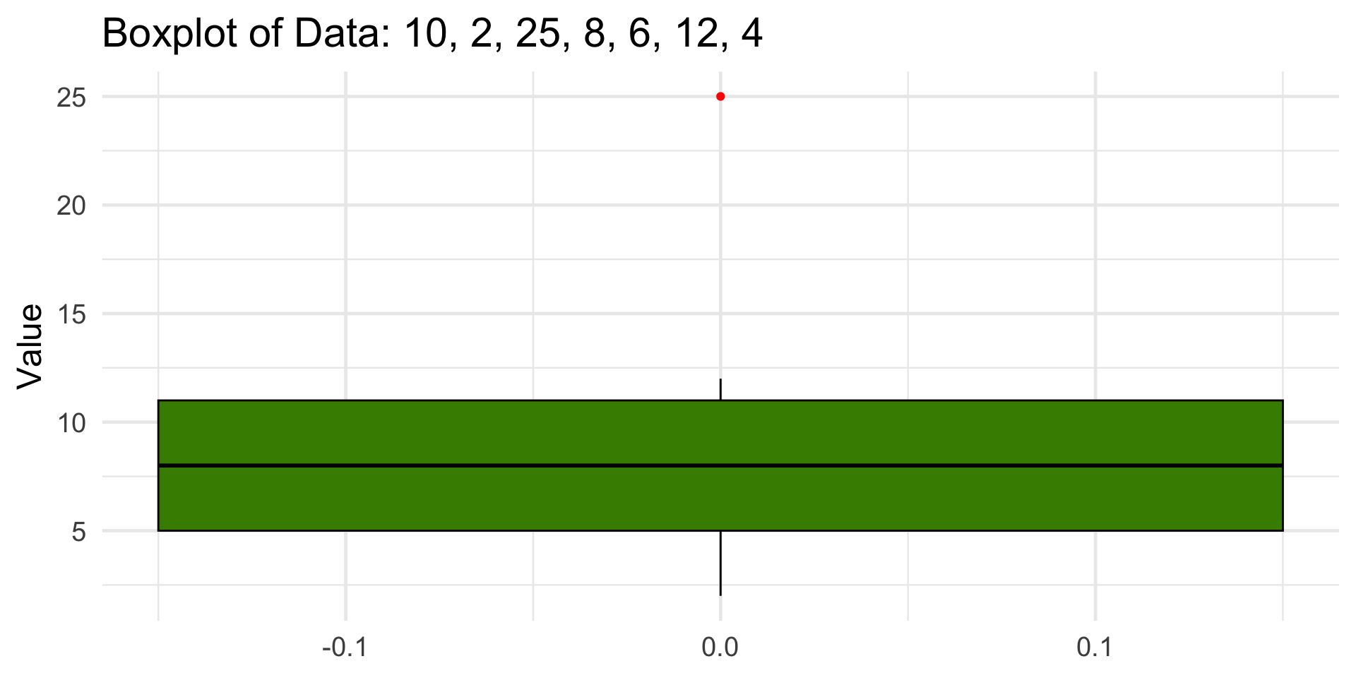
Visualizing Outliers
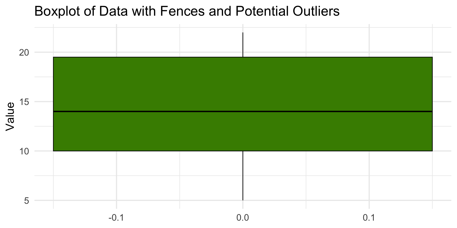
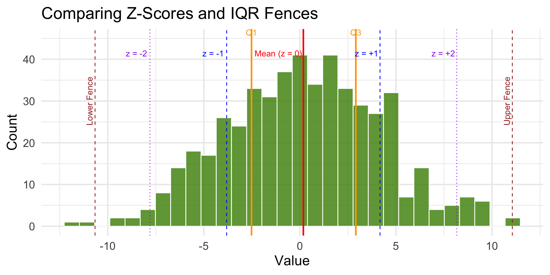
This dataset has no outliers, since all points fall between the fences (–4.25, 33.75).
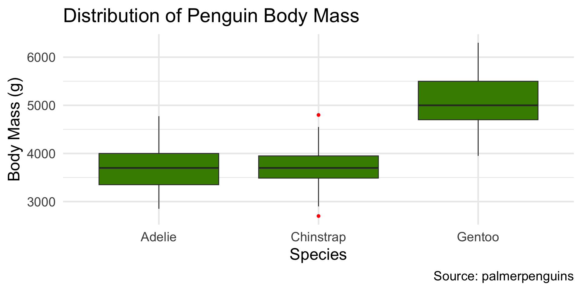
Boxplots good for comparing distributions across categories
Visual Comparison
Code
library(patchwork)
x <- tibble(x = rnorm(1000, mean = 0, 2))
a <- ggplot(x, aes(x = x )) +
  geom_histogram(binwidth = .5, fill = "chartreuse4") + theme_bw(base_size = 14) +
  geom_vline(xintercept = mean(x$x), color = "red", linewidth = 1) +
  geom_vline(xintercept = mean(x$x) - sd(x$x), color = "blue", linetype = "dashed") +
  geom_vline(xintercept = mean(x$x) + sd(x$x), color = "blue", linetype = "dashed") +
   labs(
    x = "Value",
    y = "Count",
    title = "A Distribution with Mean = 0, SD = 2"
  ) + xlim(-20, 20)
x <- tibble(x = rnorm(1000,mean = 0, 10))
b <- ggplot(x, aes(x = x )) +
  geom_histogram(binwidth = .5, fill = "chartreuse4") + theme_bw(base_size = 14) +
  geom_vline(xintercept = mean(x$x), color = "red", linewidth = 1) +
  geom_vline(xintercept = mean(x$x) - sd(x$x), color = "blue", linetype = "dashed") +
  geom_vline(xintercept = mean(x$x) + sd(x$x), color = "blue", linetype = "dashed") +
   labs(
    x = "Value",
    y = "Count",
    title = "A Distribution with Mean = 0, SD = 10"
  ) + xlim(-20, 20)
a + b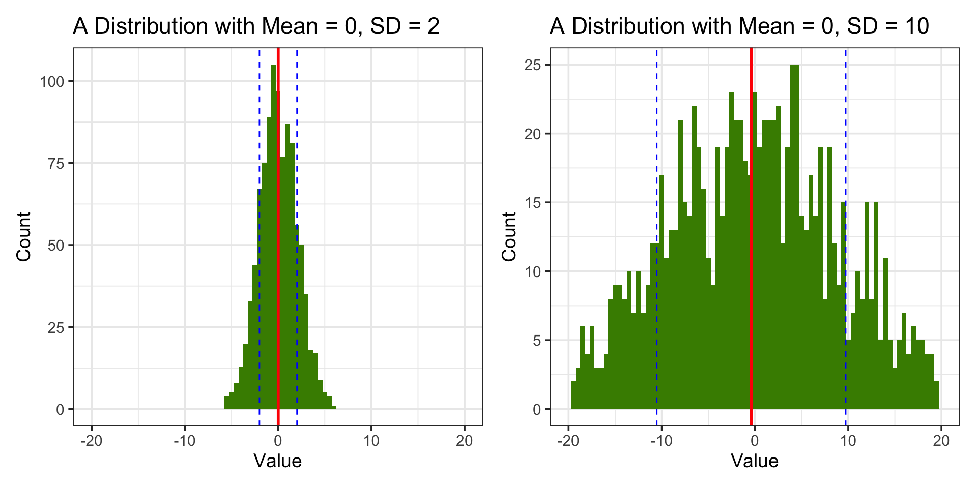
Visual Example
Code
library(ggplot2)
set.seed(7)
data <- tibble(x = rnorm(500, mean = 0, sd = 4))

mean_x <- mean(data$x)
sd_x <- sd(data$x)

ggplot(data, aes(x)) +
  geom_histogram(bins = 30, fill = "chartreuse4", color = "white", alpha = 0.8) +
  geom_vline(xintercept = mean_x, color = "red", linewidth = 1) +
  geom_vline(xintercept = mean_x + c(-1, 1) * sd_x, color = "blue", linetype = "dashed") +
  geom_vline(xintercept = mean_x + c(-2, 2) * sd_x, color = "purple", linetype = "dotted") +
  labs(
    title = "Standard Normal Distribution with Z-Scores",
    x = "Value",
    y = "Count"
  ) +
  theme_minimal(base_size = 18) + annotate("text", x = mean_x -1.3, y = 40, label = "Mean (z = 0)", color = "red", vjust = -0.5) +
  annotate("text", x = mean_x + sd_x -.7 , y = 40, label = "z = +1", color = "blue", vjust = -0.5) +
  annotate("text", x = mean_x - sd_x -.7, y = 40, label = "z = -1", color = "blue", vjust = -0.5) +
  annotate("text", x = mean_x + 2 * sd_x -.7, y = 40, label = "z = +2", color = "purple", vjust = -0.5) +
  annotate("text", x = mean_x - 2 * sd_x - .7, y = 40, label = "z = -2", color = "purple", vjust = -0.5)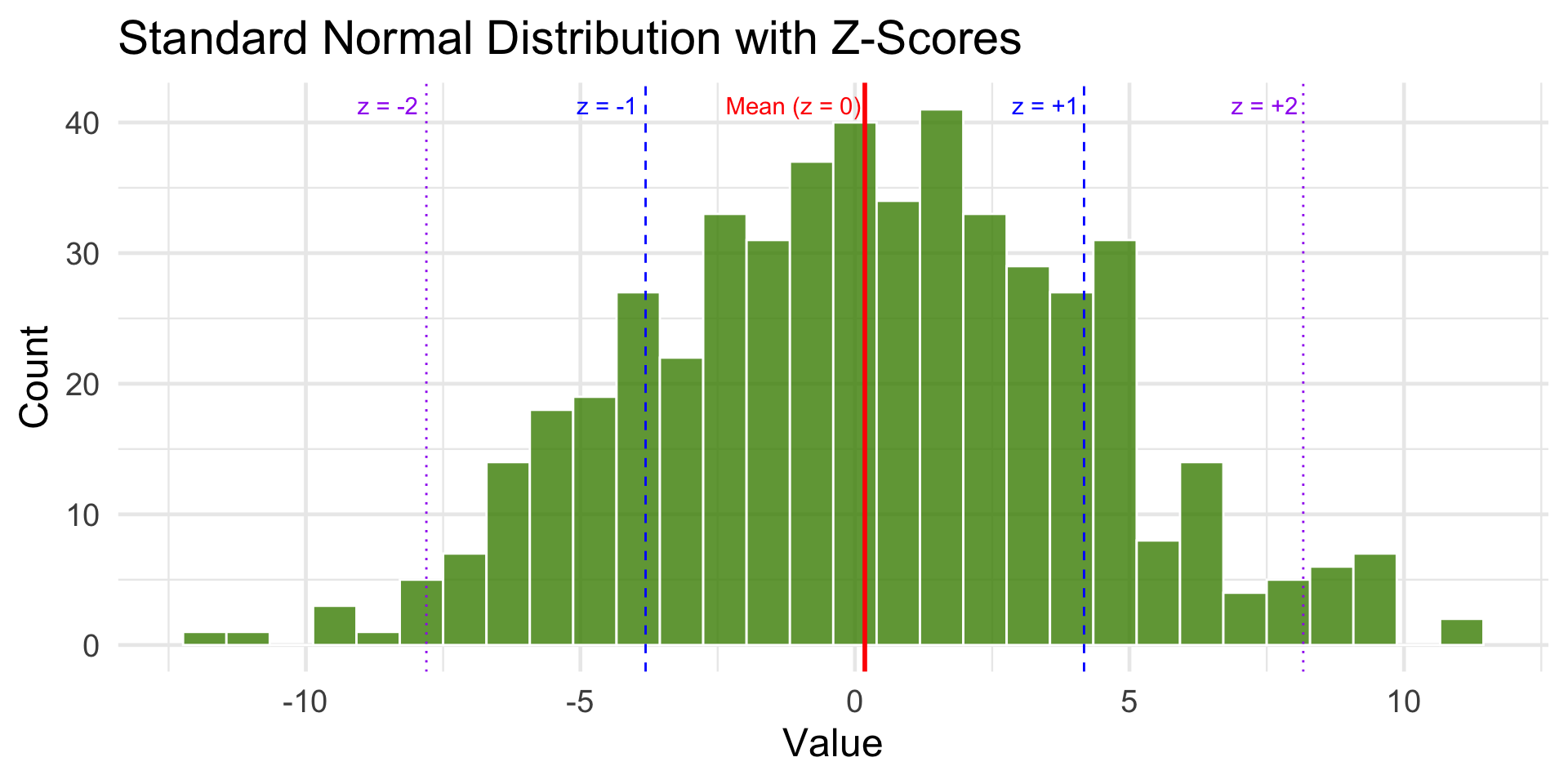
Visual Example: Z-score vs. IQR
Code
library(ggplot2)
library(dplyr)

set.seed(7)
data <- tibble(x = rnorm(500, mean = 0, sd = 4))

# Mean and standard deviation (for z-scores)
mean_x <- mean(data$x)
sd_x <- sd(data$x)

# Median and IQR (for fences)
Q1 <- quantile(data$x, 0.25)
Q3 <- quantile(data$x, 0.75)
IQR_val <- IQR(data$x)
lower_fence <- Q1 - 1.5 * IQR_val
upper_fence <- Q3 + 1.5 * IQR_val

ggplot(data, aes(x)) +
  geom_histogram(bins = 30, fill = "chartreuse4", color = "white", alpha = 0.8) +

  # Mean and z-score lines
  geom_vline(xintercept = mean_x, color = "red", linewidth = 1) +
  geom_vline(xintercept = mean_x + c(-1, 1) * sd_x, color = "blue", linetype = "dashed") +
  geom_vline(xintercept = mean_x + c(-2, 2) * sd_x, color = "purple", linetype = "dotted") +

  # IQR and fence lines
  geom_vline(xintercept = c(Q1, Q3), color = "orange", linetype = "solid", linewidth = 1) +
  geom_vline(xintercept = c(lower_fence, upper_fence), color = "brown", linetype = "dashed") +

  labs(
    title = "Comparing Z-Scores and IQR Fences",
    x = "Value",
    y = "Count"
  ) +
  theme_minimal(base_size = 18) +

  # Z-score annotations
  annotate("text", x = mean_x -1.3, y = 40, label = "Mean (z = 0)", color = "red", vjust = -0.5) +
  annotate("text", x = mean_x + sd_x - .7 , y = 40, label = "z = +1", color = "blue", vjust = -0.5) +
  annotate("text", x = mean_x - sd_x - .7, y = 40, label = "z = -1", color = "blue", vjust = -0.5) +
  annotate("text", x = mean_x + 2 * sd_x - .7, y = 40, label = "z = +2", color = "purple", vjust = -0.5) +
  annotate("text", x = mean_x - 2 * sd_x - .7, y = 40, label = "z = -2", color = "purple", vjust = -0.5) +

  # IQR annotations
  annotate("text", x = Q1, y = 45, label = "Q1", color = "orange", vjust = -0.5) +
  annotate("text", x = Q3, y = 45, label = "Q3", color = "orange", vjust = -0.5) +
  annotate("text", x = lower_fence, y = 30, label = "Lower Fence", color = "brown", angle = 90, vjust = -0.4) +
  annotate("text", x = upper_fence, y = 30, label = "Upper Fence", color = "brown", angle = 90, vjust = -0.4)