Sampling and Uncertainty

Sarah Cassie Burnett

October 23, 2025

Sampling

Sampling the act of selecting a subset of individuals, items, or data points from a larger population to estimate characteristics or metrics of the entire population
Versus a census, which involves gathering information on every individual in the population
Why would you want to use a sample?

Target Population

In data analysis, we are usually interested in saying something about a Target Population.

How many US college students check social media during their classes?
- Target population: US college students
What is the average time students spend commuting to campus each day?
- Target population: College students who attend in-person classes
What is the average number of fries in a small order at McDonald’s?
- Target population: all small fry orders at McDonald’s.

Sample

In many instances, we have a sample to talk about

We cannot talk to all college students
We cannot monitor all french fry orders

Parameters vs Statistics

The parameter is the value of a calculation for the entire target population
The statistic is what we calculate on our sample
- We calculate a statistic in order to say something about the parameter

Inference

Inference—The act of “making a guess” about some unknown
Statistical inference—Making a good guess about a population from a sample
Causal inference—Did X cause Y?

Uncertainty

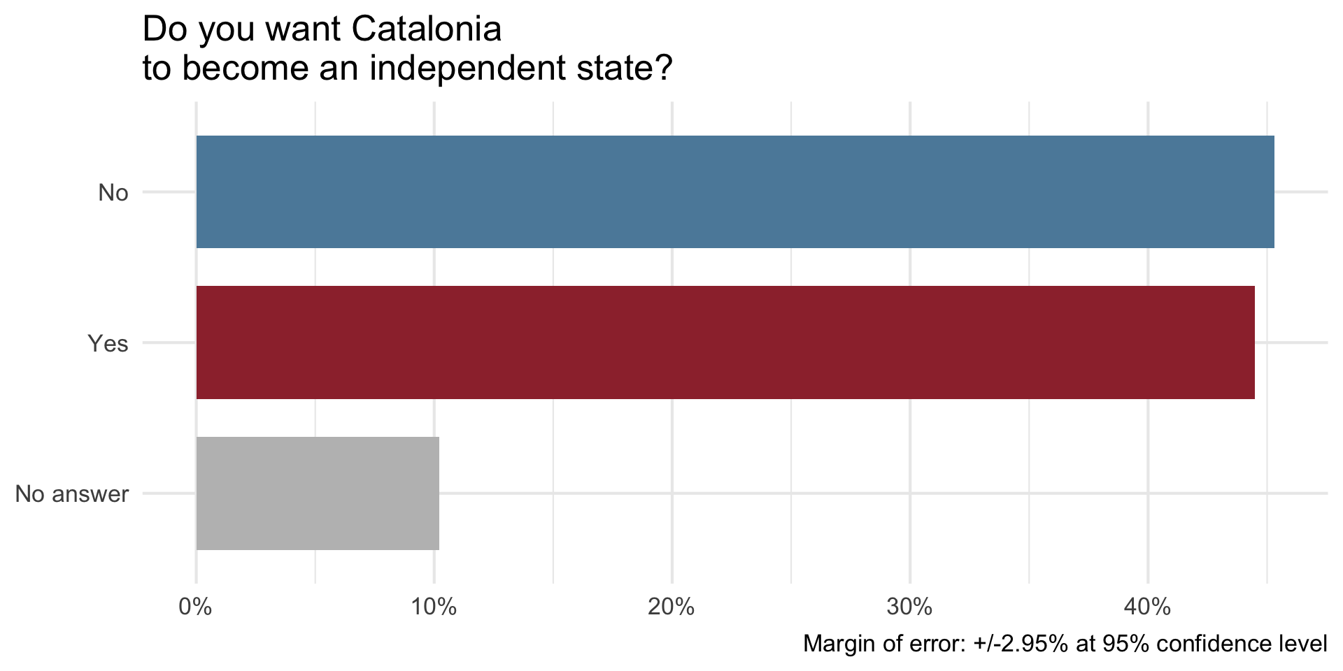
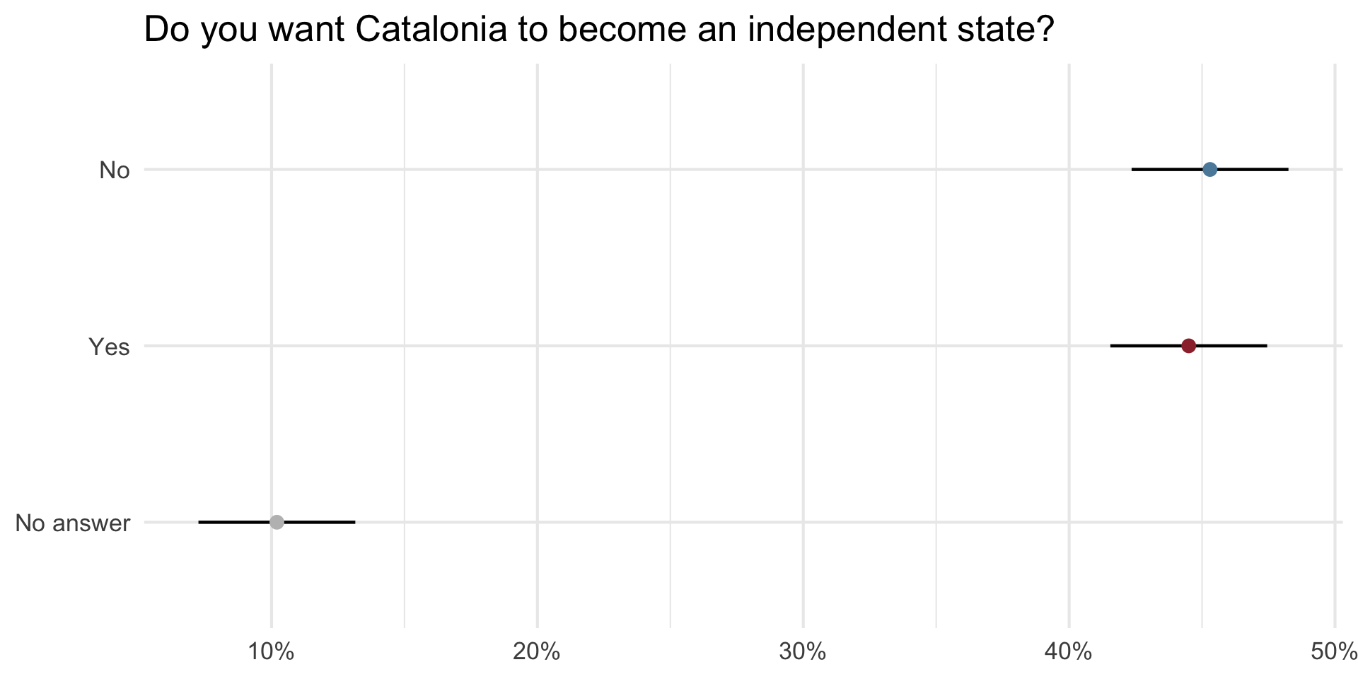
On December 19, 2014, the front page of Spanish national newspaper El País read “Catalan public opinion swings toward ‘no’ for independence, says survey”.¹

The probability of the tiny difference between the ‘No’ and ‘Yes’ being just due to random chance is very high.¹

Characterizing Uncertainty

Even unbiased procedures do not get the “right” answer every time
Estimates vary from sample to sample due to random chance
Therefore we report our estimate and our uncertainty

Solution: Create a Confidence Interval

A plausible range of values for the population parameter is a confidence interval.

95% confidence interval is standard:
- We are 95% confident that the parameter value falls within the interval

Ways to Estimate

Using math (via the Central Limit Theorem)
Using simulation (bootstrapping)

With Math…

\[CI = \bar{x} \pm Z \left( \frac{\sigma}{\sqrt{n}} \right)\]

$\bar{x}$ is the sample mean,
$Z$ is the Z-score corresponding to the desired level of confidence
$\sigma$ is the population standard deviation, and
$n$ is the sample size

We rarely have the true $\sigma$…

This part here represents the standard error:

\[\left( \frac{\sigma}{\sqrt{n}} \right)\]

Standard deviation of the sampling distribution
Characterizes the spread of the sampling distribution
The bigger this is the bigger the CIs are going to be

Common Z-values

Confidence Level	Z-Value (±)
80%	1.28
90%	1.645
95%	1.96
99%	2.576

Central Limit Theorem

Confidence Interval (CI)

\[CI = \bar{x} \pm Z \left( \frac{\sigma}{\sqrt{n}} \right)\]

This way of doing things depends on the Central Limit Theorem
As sample size gets bigger, the spread of the sampling distribution gets narrower
The shape of the sampling distributions becomes more normally distributed

Estimating Uncertainty with Confidence Intervals

A confidence interval gives us a range of plausible values for a population parameter.

A 95% confidence interval means that if we repeated our sampling many times,

Visual showing most confidence intervals covering the true mean

Conceptual Example: Student Screen Time

Suppose we survey 100 students about their average daily screen time (in hours).

Sample mean = 6.2 hours
Standard deviation = 1.5 hours
Standard error = 1.5 / √100 = 0.15

The 95% confidence interval is:

\[ 6.2 \pm 1.96 \times 0.15 = (5.91, 6.49) \]

We are 95% confident that the true average daily screen time among all students is between 5.9 and 6.5 hours.

Confidence Interval

\[CI = \bar{x} \pm Z \left( \frac{\sigma}{\sqrt{n}} \right)\]

This is therefore a parametric method of calculating the CI. It depends on assumptions about the normality of the distribution — that we know the parameters $\sigma$ and $\bar{x}$.

Bootstrapping

Use the data you have to approximate the sampling distribution
Take many with-replacement resamples of size (n)
Compute the statistic each time (mean/median/prop/etc.)
Use the middle XX% of the bootstrap statistics for the CI (e.g., 95%)
This is nonparametric—no normality assumption required

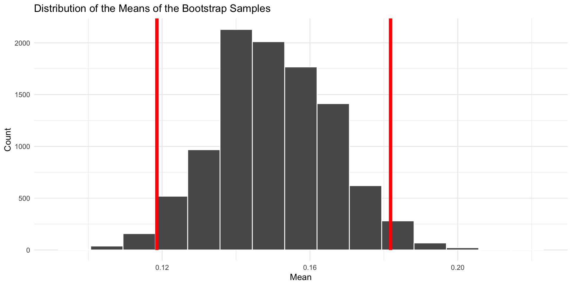
Bootstrap Process

Take a bootstrap sample - a random sample taken with replacement from the original sample, of the same size as the original sample

Calculate the bootstrap statistic - a statistic such as mean, median, proportion, slope, etc. computed on the bootstrap samples

Repeat steps (1) and (2) many times to create a bootstrap distribution - a distribution of bootstrap statistics

Calculate the bounds of the XX% confidence interval as the middle XX% of the bootstrap distribution (usually 95 percent confidence interval)

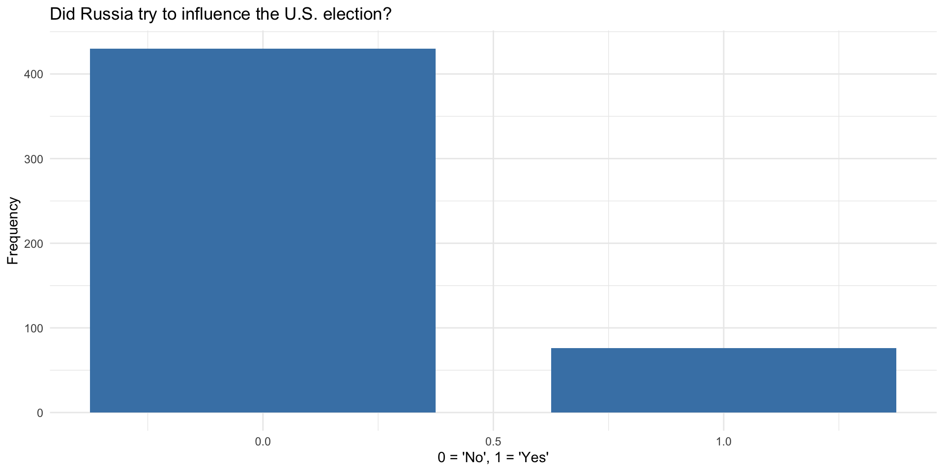
Russia

What Proportion of Russians believe their country interfered in the 2016 presidential elections in the US?

Pew Research survey
506 subjects
Data available in the openintro package

For this example, we will use data from the Open Intro package. Install that package before running this code chunk.

#install.packages("openintro")
library(openintro)

glimpse(russian_influence_on_us_election_2016)

Rows: 506
Columns: 1
$ influence_2016 <chr> "Did not try", "Did not try", "Did not try", "Don't kno…

Let’s use mutate() to recode the qualitative variable as a numeric one…

russiaData <- russian_influence_on_us_election_2016 |> 
  mutate(try_influence = ifelse(influence_2016 == "Did try", 1, 0))

Now let’s calculate the mean and standard deviation of the try_influence variable…

russiaData |>
  summarize( 
          mean = mean(try_influence),
          sd = sd(try_influence)
  )

# A tibble: 1 × 2
   mean    sd
  <dbl> <dbl>
1 0.150 0.358

And finally let’s draw a bar plot…

ggplot(russiaData, aes(x = try_influence)) +
  geom_bar(fill = "steelblue", width = .75) +
  labs(
    title = "Did Russia try to influence the U.S. election?",
    x = "0 = 'No', 1 = 'Yes'",
    y = "Frequency"
  ) +
  theme_minimal()

Bootstrap with `tidymodels`

Install tidymodels before running this code chunk…

#install.packages("tidymodels")
library(tidymodels)

set.seed(66)
boot_dist <- russiaData |>
  specify(response = try_influence) |>          # specify the variable of interest
  generate(reps = 10000, type = "bootstrap") |> # generate 10000 bootstrap samples
  calculate(stat = "mean")                      # calculate the mean of each bootstrap sample

glimpse(boot_dist)

Rows: 10,000
Columns: 2
$ replicate <int> 1, 2, 3, 4, 5, 6, 7, 8, 9, 10, 11, 12, 13, 14, 15, 16, 17, 1…
$ stat      <dbl> 0.1146245, 0.1442688, 0.1343874, 0.1877470, 0.1521739, 0.138…

Calculate the mean of the bootstrap distribution (of the means of the individual draws)…

boot_dist |> summarize(mean = mean(stat))

# A tibble: 1 × 1
   mean
  <dbl>
1 0.150

Calculate the confidence interval. A 95% confidence interval is bounded by the middle 95% of the bootstrap distribution.

boot_dist |>
  summarize(lower = quantile(stat, 0.025),
            upper = quantile(stat, 0.975))

# A tibble: 1 × 2
  lower upper
  <dbl> <dbl>
1 0.119 0.182

Create upper and lower bounds for visualization.

# for using these values later
lower_bound <- boot_dist |> summarize(lower_bound = quantile(stat, 0.025)) |> pull() 
upper_bound <- boot_dist |> summarize(upper_bound = quantile(stat, 0.975)) |> pull()

Visualize with a histogram

ggplot(data = boot_dist, mapping = aes(x = stat)) +
  geom_histogram(binwidth =.01, fill = "steelblue4") +
  geom_vline(xintercept = c(lower_bound, upper_bound), color = "darkgrey", size = 1, linetype = "dashed") +
  labs(title = "Bootstrap distribution of means",
       subtitle = "and 95% confidence interval",
       x = "Estimate",
       y = "Frequency") +
  theme_bw()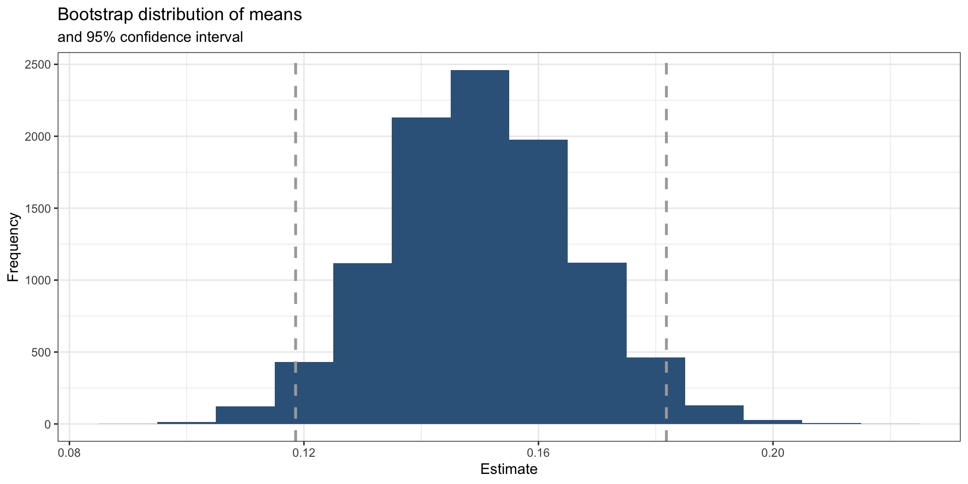

Or use the `infer` package

ci <- boot_dist |> get_ci(level = 0.95) 

ci

# A tibble: 1 × 2
  lower_ci upper_ci
     <dbl>    <dbl>
1    0.119    0.182

Or use the `infer` package

boot_dist |>
  visualize() +
  shade_ci(ci, color = "red", fill = NULL) +
  labs( 
    title = "Distribution of the Means of the Bootstrap Samples",
    x = "Mean",
    y = "Count"
  ) +
  theme_minimal()

Or use the `infer` package

boot_dist |>
  visualize() +
  shade_ci(ci, color = "red", fill = NULL) +
  labs( 
    title = "Distribution of the Means of the Bootstrap Samples",
    x = "Mean",
    y = "Count"
  ) +
  theme_minimal()

Interpret the confidence interval

The 95% confidence interval was calculated as (lower_bound, upper_bound). Which of the following is the correct interpretation of this interval?

(a) 95% of the time the percentage of Russian who believe that Russia interfered in the 2016 US elections is between lower_bound and upper_bound.

(b) 95% of all Russians believe that the chance Russia interfered in the 2016 US elections is between lower_bound and upper_bound.

(c) We are 95% confident that the proportion of Russians who believe that Russia interfered in the 2016 US election is between lower_bound and upper_bound.

(d) We are 95% confident that the proportion of Russians who supported interfering in the 2016 US elections is between lower_bound and upper_bound.

Interpret the confidence interval

The 95% confidence interval was calculated as (lower_bound, upper_bound). Which of the following is the correct interpretation of this interval?

(c) We are 95% confident that the proportion of Russians who believe that Russia interfered in the 2016 US election is between lower_bound and upper_bound.

Try it out!

Given that the mean of 0-1 encoded data is equal to the proportion, use the following formula to estimate the confidence interval based on the sample of 506 Russians,

03:00

We estimate the standard error using:

\[ SE = \sqrt{ \frac{ \hat{p}(1 - \hat{p}) }{n} } \]

Tips:

To count rows: nrows(your_data)
To access a column in a data frame: your_data$col_name

Why did we do these simulations?

They provide a foundation for statistical inference and for characterizing uncertainty in our estimates
The best research designs will try to maximize or achieve good balance on bias vs precision

Sampling and Uncertainty

Sampling

Target Population

Sample

Parameters vs Statistics

Inference

Uncertainty

Characterizing Uncertainty

Solution: Create a Confidence Interval

Ways to Estimate

With Math…

Common Z-values

Central Limit Theorem

Confidence Interval (CI)

Estimating Uncertainty with Confidence Intervals

Conceptual Example: Student Screen Time

Confidence Interval

Bootstrapping

Bootstrap Process

Russia

Bootstrap with tidymodels

Or use the infer package

Or use the infer package

Or use the infer package

Interpret the confidence interval

Interpret the confidence interval

Try it out!

Why did we do these simulations?

Bootstrap with `tidymodels`

Or use the `infer` package

Or use the `infer` package

Or use the `infer` package